Loading STL files and calculating the loaded state of the turbine blade
In this script, we will show an example of how to use Engee environment.:
- upload a three-dimensional model of a part from the STL format
- Visualize the grid of this model
- calculate the loaded state of the part using MATLAB commands
To open a CAD file (in STL format), we will use the library [Meshes.jl](https://juliageometry.github.io/Meshes .jl/stable/). It allows you to work with many different CAD formats and computational grids and can prepare a saved 3D model of an object for further manipulation.
For visualization, we first use the standard Plots library built into Engee, then the higher–level [Makie] library (https://docs.makie.org/stable /). You can evaluate its capabilities by visiting Makie Graphics Gallery.
In the third part, we will demonstrate how an example of calculating the mechanical load experienced by a turbine blade can be performed in Engee and visualize the graphs.
Uploading a three-dimensional model
First, we will connect the necessary libraries for this stage.
Pkg.add(["CairoMakie", "Makie", "Animations", "Meshes", "MeshIO"])
import Pkg; Pkg.add(["Meshes", "MeshIO"], io=devnull);
using Meshes, MeshIO, FileIO, Plots
# plotly();
gr();
We will specify a working folder for all future file operations.
cd( @__DIR__ )
Now let's load the model and display the calculated grid on the graph using separate triangles, each of which can be styled individually in any way.
obj = load( "Blade.stl" );

p = plot()
for i in obj
    m = Matrix([i[1] i[2] i[3] i[1]])'
    plot!( p, m[:,1], m[:,2], m[:,3], lc=:black, label=:none, lw=.1 )
end
plot!( camera=(120, 30), axis=nothing, border=:none, aspect_ratio=:equal, projection_type=:persp )
display(p)
Why don't we draw a three-dimensional animation of the rotation of this part?
Pkg.add( "Animations", io=devnull );
using Animations
obj = load( "Blade.stl" );

@gif for az in 0:10:359
    p = plot()
    for i in obj
        m = Matrix([i[1] i[2] i[3] i[1]])'
        plot!( p, m[:,1], m[:,2], m[:,3], lc=:black, label=:none, lw=.1 )
    end
    plot!( camera = (az, 30), axis=nothing, border=:none, aspect_ratio=:equal )
end
To demonstrate a high-level method of working with the model, we will connect the library for visualization. Makie, and we will choose a suitable toolkit for fast graph rendering (CairoMakie). Another option supported by the browser is the package WGLMakie, requires more complex settings. Other packages (GLMakie and RPRMakie) require the creation of additional windows and are not yet supported by Engee.
import Pkg; Pkg.add(["Makie", "CairoMakie"], io=devnull);
using Makie, CairoMakie
Visualize the model in one line.
The first execution of this cell, immediately after loading the Makie library, may take more than a minute.
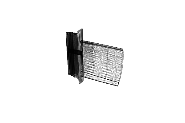
Makie.wireframe( obj, linewidth=.2 )

Let's perform calculations using the MATLAB kernel
To calculate using finite element methods, as a rule, you need to use well-established external tools. There are many excellent research packages in this field. For example, packages for dividing a grid into polygons (tetgen, gmsh) there are shells in Julia that can be connected to Engee to perform calculations.
If you already have an existing project in MATLAB, or you have found a demo code that is very similar to what you need, then Engee will allow you to run it and save the result to the cloud.
using MATLAB
Let's set a calculation problem and upload a three-dimensional model of the part.
The first execution of this cell, immediately after connecting the MATLAB library, may take more than a minute._
mat"cd $(@__DIR__)"
outp = mat"""
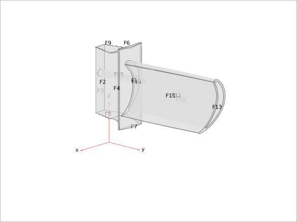
smodel = createpde('structural','static-solid');
g = importGeometry(smodel, 'Blade.stl');
figure;
p = pdegplot( smodel, 'FaceLabels', 'on', 'FaceAlpha',0.5);
axis off;
view( [133.027 16.056] );
saveas( gcf, 'Blade.png' );
""";
We will display the saved image in the Engee environment using the command load built into the Engee library Images.
using Images
img = Images.load( "Blade.png" )
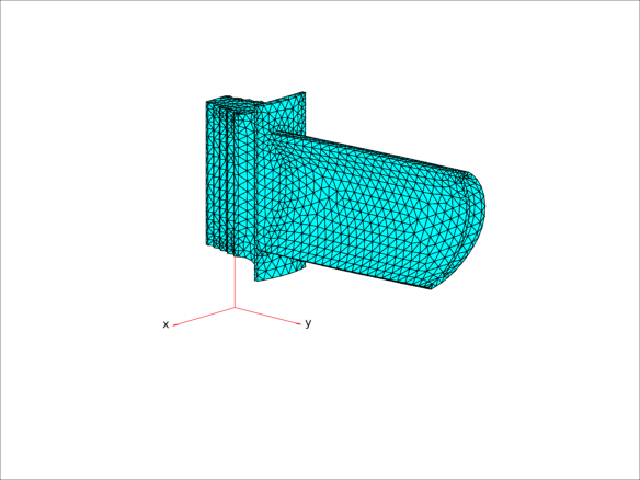
The uploaded file contained only a description of the surface. Now let's create a three-dimensional computational grid inside this surface.
outp = mat"""
msh = generateMesh(smodel,'Hmax',0.01);

figure
p1 = pdemesh(msh, 'FaceAlpha', 1)
view([133.027 16.056])

saveas( gcf, "Blade_mesh.png" )
""";
img = Images.load( "Blade_mesh.png" )
And thirdly, we need to set the parameters of the problem (computational and physical), in particular the boundary conditions.
Calculate the blade deformation using the function solve and we will display a three-dimensional graph on which the mechanical deformation of the part will be amplified hundreds of times, and the color information will show the degree of mechanical stress in the circumference of this point of the part.
outp = mat"""
E = 227E9; % in Pa
CTE = 12.7E-6; % in 1/K
nu = 0.27;

s1 = structuralProperties(smodel,'YoungsModulus',E, ...
                            'PoissonsRatio',nu, ...
                            'CTE',CTE);

s2 = structuralBC(smodel,'Face',3,'Constraint','fixed');

p1 = 5e5; %in Pa
p2 = 4.5e5; %in Pa

s3 = structuralBoundaryLoad(smodel,'Face',11,'Pressure',p1); % Pressure side
s4 = structuralBoundaryLoad(smodel,'Face',10,'Pressure',p2);  % Suction side

Rs = solve(smodel);

figure
p2 = pdeplot3D(smodel,'ColorMapData',Rs.VonMisesStress, ...
                 'Deformation',Rs.Displacement, ...
                 'DeformationScaleFactor',100);
%view([116,25]);
view( [133.027 16.056] );

saveas(gcf, "Blade_solved.png");
""";
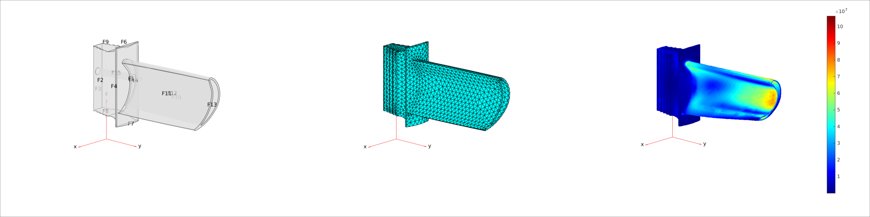
Let's display two graphs in the same projection: the first one shows the distribution of the blade zones for which we set the boundary conditions. The second one shows a deformed model with marked areas of high mechanical stress.
img_topo = Images.load( "Blade.png" );
img_mesh = Images.load( "Blade_mesh.png" );
img_solved = Images.load( "Blade_solved.png" );
mosaic(img_topo, img_mesh, img_solved; nrow=1)