Calculation of the temperature field of a flat radiation heat exchanger
Determination of heat exchanger parameters, design scheme, initial and boundary conditions
In this example, the solution of the heat conduction equation by the Euler method will be demonstrated.
Task: Calculate the temperature field for a flat radiation heat exchanger.
Given:
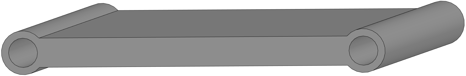
The flat radiation heat exchanger is 20 cm long and 1.25 cm thick.
Initial conditions:
The vacuum,
the integral absorption capacity of the body ,
spectral absorption capacity of the body ,
the temperature at each point of the heat exchanger at the initial time .
Boundary conditions:
temperature of the coolant .
Assumptions:
heat transfer along the liquid flow is not taken into account, and therefore the width of the heat exchanger is assumed to be 1 cm.,
The radiation from only one side of the heat exchanger is taken into account, since the other side absorbs the heat re-reflected from the cooled spacecraft.
The general view of the heat exchanger is shown in the figure:
The classical equation of thermal conductivity has been modified to take into account radiant heat exchange with the environment, which is described by the Stefan-Boltzmann law.
Applying the Euler method to this equation, we obtained:
where:
(J/kg*K) is the heat capacity of aluminum,
kg is the mass of the calculated heat exchanger section.,
W/(m*K) is the coefficient of thermal conductivity,
m2 - the area of the calculated plot,
m is the length of the calculated section of the heat exchanger,
- the integral absorption capacity of the body,
W/(m2*K4);
- the area of the midsection of the calculated area (projection of the area of the site perpendicular to the direction of solar radiation)
- spectral absorption capacity of the body,
W/m2 is the intensity of solar radiation,
c is the calculation step.
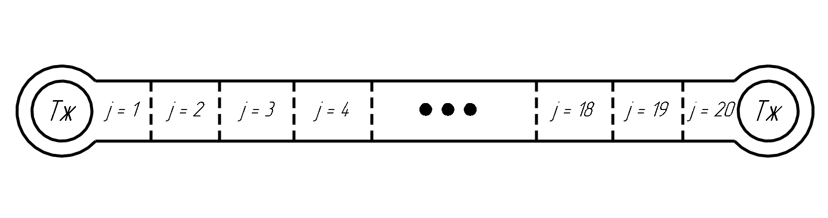
The location of the calculated segments is shown in the figure:
Determination of initial conditions, parameters of the heat exchanger and the environment
Determination of heat exchanger and environmental parameters:
# @markdown #### Selection of heat exchanger material with a certain heat capacity (in order: aluminum, iron, gold)
c = "903.7" # @param ["903.7", "450.0", "130.0"]
c = parse(Float64, c)
m = 0.003375
A = 235.9
F = 0.00025
d = 0.01
E = 0.90
S = 0.000000056704
Fm = F*sin(67*pi/180)
L = 0.14
# @markdown #### Determination of heat flow from the sun (sunny side/shadow)
q = "1400.0" # @param ["1400.0", "0.0"]
q = parse(Float64, q)
# @markdown #### Defining the calculation step by time
h = 0.1 # @param {type:"number"}
Calculation and visualization of data
Plotting the time decision for segments 1 to 10 (from the left edge to the middle of the heat exchanger):
using Plots
# Determining the initial conditions
T0 = 293.15
T = fill(293.0, (1080,20)); # defining an array for temperature
Q3 = fill(0.094, (1080,20)); # determination of the array for the heat flow emitted by the heat exchanger
Q4 = fill(0.0451047, (1080,20)); # definition of an array for the heat flow radiated by the Sun

# Calculation of temperatures and heat fluxes at each time point
# for all segments of the heat exchanger:
for i in 1:1079 # time calculation cycle
    # @markdown #### Coolant temperature on the left:
    T[i,1] = 290.06 # @param {type:"slider", min:250, max:350, step:0.01}
    # @markdown #### Coolant temperature on the right:
    T[i,20] = 293.13  # @param {type:"slider", min:250, max:350, step:0.01}
        for j in 2:19 # a cycle for calculating the coordinate
            T[1,j] = T0 # defining the initial condition
            T[i+1,j] = T[i,j] + h*(
                (1/(c*m))*
                (A*F*(T[i,j-1]-T[i,j])/d # the heat flow transferred from the left segment to the current one by thermal conduction
                 + A*F*(T[i,j+1]-T[i,j])/d # the heat flow transferred from the right segment to the current one by thermal conduction
                 - E*S*T[i,j]*T[i,j]*T[i,j]*T[i,j]*F # heat flow radiated by the current section of the heat exchanger
                 + L*q*Fm) # heat flow from the Sun absorbed by the current section of the heat exchanger
                 )
            Q3[i,j] = E*S*T[i,j]*T[i,j]*T[i,j]*T[i,j]*F # filling the array for the radiated heat flow
            Q4[i,j] = L*q*Fm # filling the array for the absorbed heat flow
        end
end
T[end,1] = T[end-1,1]
Legend = ["1 segment" "2 segment" "3 segment" "4 segment" "5 segment" "6 segment" "7 segment" "8 segment" "9 segment" "10 segment"]
# plotting graphs for segments 11 through 20 does not make sense, since they are geometrically symmetric with segments 1 through 10.
Plots.plot(T[:,1:10], xlabel="Time", ylabel="Temperature", label=Legend) # , ylims=(lim_low,lim_high)
Conclusions:
In this example, the calculation of the temperature field of a flat heat exchanger was demonstrated. From the calculation of the ratio of radiated and absorbed heat fluxes, it can be seen that the heat exchanger actually absorbs the heat brought by the coolant and radiates it into the environment. In turn, depending on the coordinate, the temperature values were obtained at each time point. Thus, the problem of calculating the temperature field in a flat heat exchanger was solved.