Calculation of the stationary thermal field in detail: Julia, Gmsh, Gridap, VTK and Makie
Let's apply a chain of tools that allows Engee to design, parameterize a model, apply a computational grid to it, build a problem for solving using the finite element method and, as a result, calculate heat transfer in a complex part.
Introduction
For problems requiring precise solutions of partial differential equations (for example, heat transfer or deformable body mechanics), specialized tools (such as Gridap or FEniCS) provide more accurate and flexible results. They allow you to work with arbitrary grids and complex boundary conditions, which is critical for scientific calculations.
Pkg.add(["Gridap", "GridapGmsh", "CairoMakie", "WriteVTK", "ReadVTK", "GeometryBasics"])
For this example, we use a library, the installation of which automatically adds the Gmsh package to the system.
using GridapGmsh
Let's take a simple model example from the repository of this library and slightly modify it:
- region
boundary 1will unite the inner surface of the wider hole (on the right) - region
boundary 2- the entire inner surface of the hole with a protrusion (on the left)
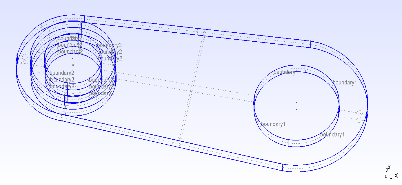
You can create such a parameterized model in a text editor, for example, by visualizing the results in https://gmsh.info / or in one of the many CAD systems for solid-state modeling, including open source ones: [OpenCascade](https://dev.opencascade.org /), [OpenSCAD](https://openscad.org /) and [FreeCAD](https://www.freecad.org /).
Let's upload an example in the * format.geo* (the basic format for geometry in Gmsh) and create a grid:
GridapGmsh.gmsh.initialize()
GridapGmsh.gmsh.clear()
GridapGmsh.gmsh.open("$(@__DIR__)/demo.geo");
GridapGmsh.gmsh.model.geo.synchronize();
GridapGmsh.gmsh.option.setNumber("Mesh.CharacteristicLengthMin", 0.01)  # minimum size
GridapGmsh.gmsh.option.setNumber("Mesh.CharacteristicLengthMax", 0.05)  # maximum size
GridapGmsh.gmsh.model.mesh.generate(3);
GridapGmsh.gmsh.write("demo.msh");
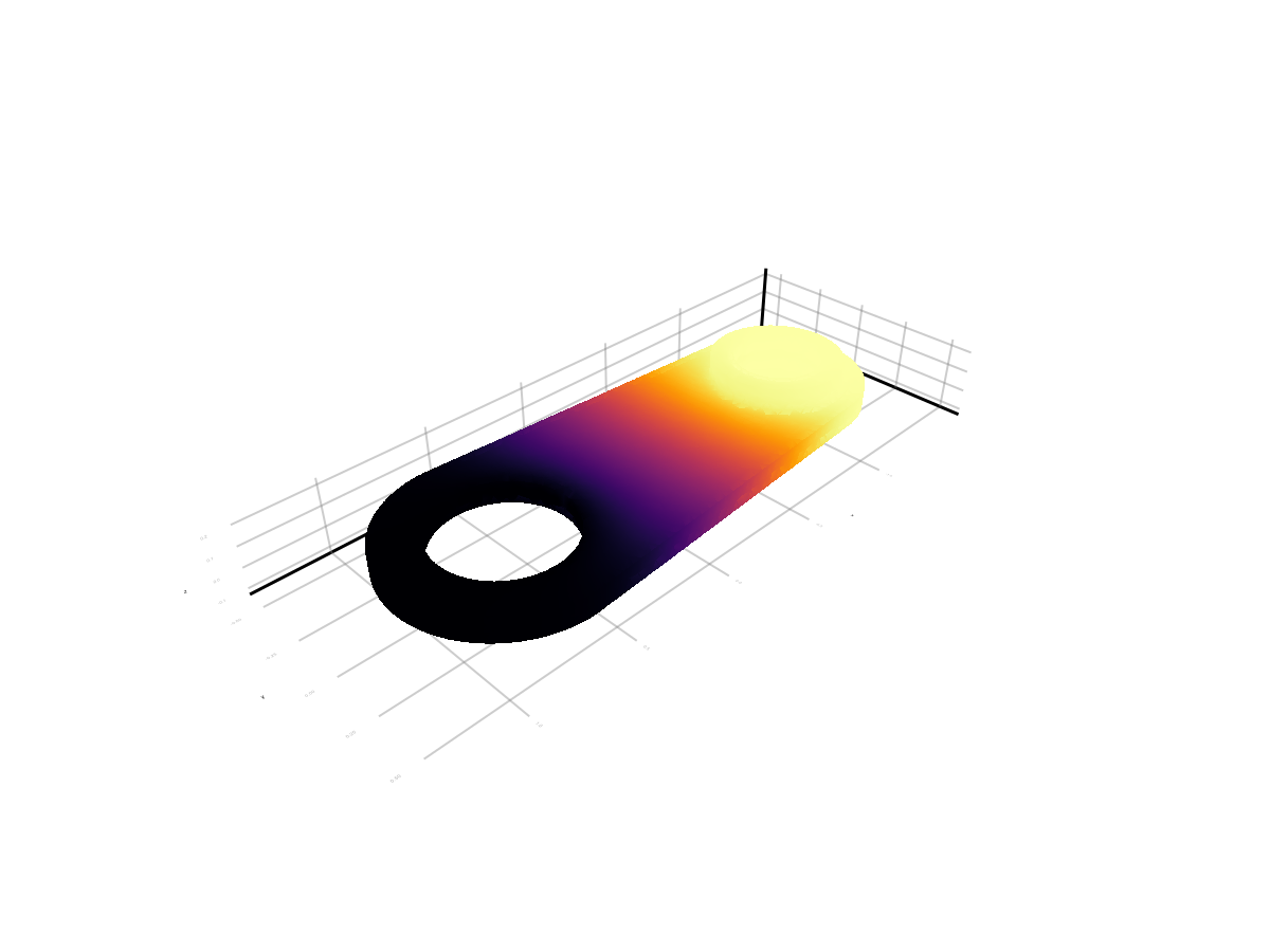
Let's print the model of our part, which is a set of tetrahedra (Makie does not allow working with tetrahedra, so we manually converted them into triangles). The color scheme of the graph corresponds to the coordinate of the points on the X-axis.
using Gridap, GridapGmsh, GeometryBasics

import CairoMakie: mesh, NoShading
# import WGLMakie: mesh, NoShading # To replace CairoMakie - for interactive charts

model = GmshDiscreteModel("demo.msh");

grid = get_grid(get_triangulation(model))
points = reinterpret(reshape, Float64, grid.node_coordinates)
cells = hcat(grid.cell_node_ids...)

tetrahedra = [ (c[1], c[2], c[3], c[4]) for c in eachcol(cells) ]
all_faces = [ [TriangleFace{Int}(ta, tb, tc),TriangleFace{Int}(ta, tb, td),TriangleFace{Int}(ta, tc, td),TriangleFace{Int}(tb, tc, td)] for (ta, tb, tc, td) in tetrahedra ]
all_faces = reshape(reinterpret(Int, vcat(all_faces...)), 3, :)
colors = points[1,:]

mesh(points', all_faces', color=colors, shading=NoShading)

Setting a numerical problem
We use the code from basic example for GridapGmsh, where the Laplace's equation is solved with Dirichlet boundary conditions in a weak (variational) formulation by the finite element method (FEM).
Laplace equation and boundary conditions: The function is being searched for satisfying the equation in the area of with boundary conditions on , on , where — the area defined by the grid
demo.msh, and — borders with tags "boundary1" and "boundary2" respectively.
Weak form (variational formulation of the problem) is a key method for modern FEM, it weakens the requirements for the smoothness of the solution, and boundary conditions can be set directly without approximating them. And, of course, this is the main method of discretization of the problem, which allows you to set it in basic functions and solve it as a linear system. . So, our problem in the variational formulation is transformed into , where — gradient, — the area of integration, — a test space that turns to zero at the borders.
Note how close the description given in the code is ∫( ∇(v)⋅∇(u) )dΩ towards the Laplace equation in a variational formulation .
using Gridap

model = GmshDiscreteModel("demo.msh");         # Loading the grid geometry from the *.msh file
order = 1
reffe = ReferenceFE(lagrangian,Float64,order)  # Linear Lagrangian elements of the 1st order
V = TestFESpace(model,reffe,dirichlet_tags=["boundary1","boundary2"]) # Trial space
U = TrialFESpace(V,[0,1])                      # Definition of the solution space
                                               # - on boundary1, the solution value is u = 0
                                               # - on boundary2, the value is u = 1
Ω = Triangulation(model)                       # Triangulation and integration measure
dΩ = Measure(Ω,2*order)
a(u,v) = ∫( ∇(v)⋅∇(u) )dΩ                      # The weak form of the Laplace equation
l(v) = 0                                       # Linear shape (right side)
op = AffineFEOperator(a,l,U,V)                 # We collect the linear operator of the problem
uh = solve(op)                                 # System solution

writevtk(Ω,"demo",cellfields=["uh"=>uh]);
We will go a little further and, in addition to on-the-fly visualization, we will show you how to visualize a calculation saved in VTK. But first, let's show the solution we just improved.:
using GeometryBasics
nodes = GridapGmsh.get_node_coordinates(Ω)
cell_node_ids = GridapGmsh.get_cell_node_ids(Ω)
uh_values = [uh(node) for node in nodes]
points = [Point3f(x...) for x in nodes]
faces = [TriangleFace(cell_node_ids[i][1], cell_node_ids[i][2], cell_node_ids[i][3]) for i in 1:length(cell_node_ids)]
mesh(points, faces, color=uh_values, colormap=:inferno, shading=NoShading)
Visualization of the solution from a VTK file
The most convenient solution for viewing VTK files is an open source program [ParaView](https://www.paraview.org /). But it is also valuable for us to have interactive reports that are fully open in Engee. Therefore, we will open this file in Julia and output the solution directly in this script.
If we run this part asynchronously with the solution of the problem (which may take a long time), we will need to connect these libraries.:
using WriteVTK, ReadVTK
They will help us read the VTK file and display it on 3D graphics. There are additional libraries for some of the functions, but for now we'll make do with low-level commands.:
- create a matrix
pointsfor the coordinates of the vertices - get the vector
uh_valueswhere the field values will be locateduhour solution - let's break the tetrahedra
cellson a set of trianglesall_faces
vtk = VTKFile("demo.vtu")
points = get_points(vtk)
uh_values = get_data(get_point_data(vtk)["uh"])
cells = get_cells(vtk)
# Let's split the cells.connectivity array into tetrahedra, and then into triangles
using GeometryBasics
all_faces = TriangleFace{Int}[]
offset = 1
while offset <= length(cells.connectivity)
ta, tb, tc, td = cells.connectivity[offset:offset+3]
push!(all_faces, TriangleFace(ta, tb, tc)) # face 1
push!(all_faces, TriangleFace(ta, tb, td)) # face 2
push!(all_faces, TriangleFace(ta, tc, td)) # face 3
push!(all_faces, TriangleFace(tb, tc, td)) # face 4
offset += 4
end
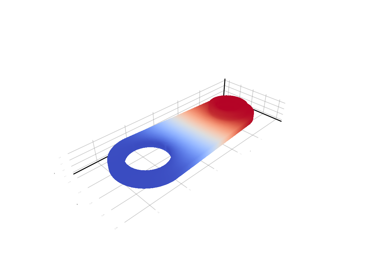
# CairoMakie does not accept the last triangle in the model, we temporarily use [1:end-1]
mesh(points, all_faces[1:end-1], color=uh_values, colormap=:coolwarm, shading=NoShading)
Conclusion
We implemented the solution of the Laplace equation on a tetrahedral grid, saved the results in VTK format and visualized them.
These are the key stages of modeling physical fields (thermal, electrical, mechanical). This approach ensures reproducibility, accuracy, and readiness to scale to real engineering tasks that require detailed calculations rather than simplified system approximations.