Population dynamics based on catch
In this example, we will show how easy it is to create and solve a differential equation that allows you to model the dynamics of a fish population based on catch.
Description of the model
We will model a fish population in a reservoir that is subject to the following processes:
- the effect of fertility and mortality is described by a quadratic function
- The catch task annually reduces the population by tons
- the initial population size is .
Thus, we create a model of the following task:
The general view of the flowchart, which can be used to model this task, is as follows:
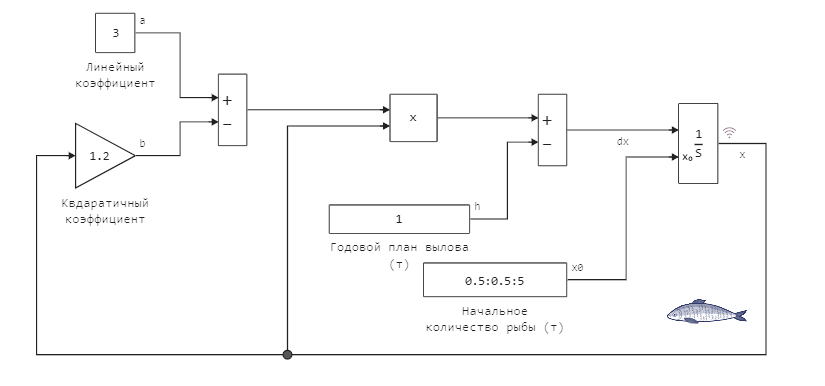
All parameters are easily accessible, and they can be set both from the script (via variables) and on the canvas itself. Numerical integration will help us solve this system, but it's worth remembering:
-
there are combinations of input conditions that make the solution unstable (the population goes into );
-
in case of instability, the constant-step solver may not report an error, therefore, the variable-step solver is selected in the model settings.;
-
The maximum simulation step size is set to 0.01, so that the interval is 0..1 we still got a smooth schedule, even if we can take longer steps according to the conditions of the task.
Launching and analyzing the results
Let's run the model using software management tools:
# We will load the model if it is not already open on the canvas.
if "fish_population_diff_eq_model" ∉ getfield.(engee.get_all_models(), :name)
    engee.load( "$(@__DIR__)/fish_population_diff_eq_model.engee");
end
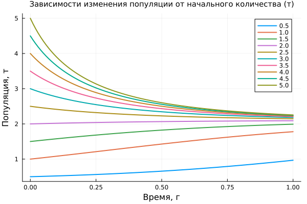
Let's plot the dependence of population dynamics on changes in its initial size.:
# Let's launch the model
model_data = engee.run( "fish_population_diff_eq_model" );

# Let's read the necessary parameters for the graph output.
param_vector = engee.get_param("fish_population_diff_eq_model/Начальное количество рыбы (т)", "Value");
param_vector = eval(Meta.parse(param_vector)); # Converting a string to a vector

plot( model_data["x"].time, hcat( model_data["x"].value... )',
      label=reshape(param_vector, 1, :), lw=2,
      title="The dependence of population change on the initial number (t)", titlefont=font(10),
      xlabel="Time, g", ylabel="Population, t" )
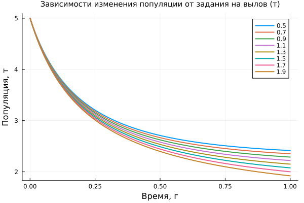
Now we will set one value x0 and we will plot a graph depending on the change in the annual catch plan.:
param_1 = engee.get_param("fish_population_diff_eq_model/Годовой план вылова (т)", "Value" );

# Changing the model parameters
engee.set_param!( "fish_population_diff_eq_model/Начальное количество рыбы (т)", "Value"=>"5.0" );
engee.set_param!( "fish_population_diff_eq_model/Годовой план вылова (т)", "Value"=>"0.5:0.2:2" );
# # Let's launch the model
model_data = engee.run( "fish_population_diff_eq_model" );
# # Get the model parameters for the graph
param_2 = engee.get_param("fish_population_diff_eq_model/Годовой план вылова (т)", "Value" );
param_2 = eval(Meta.parse(param_2));

plot( model_data["x"].time, hcat( model_data["x"].value... )',
      label=reshape(param_2, 1, :), lw=2,
      title="Dependence of population change on the catch task (t)", titlefont=font(10),
      xlabel="Time, g", ylabel="Population, t" )
And return the model to its original state.
engee.set_param!("fish_population_diff_eq_model/Годовой план вылова (т)", "Value"=>param_1 );
engee.set_param!("fish_population_diff_eq_model/Начальное количество рыбы (т)", "Value"=>string(param_vector) );
Conclusion
Solving differential equations using a flowchart and an integrator simplifies the transfer of knowledge between representatives of different specialties, as we have seen by solving the differential equation of population growth.