Discharge-battery charge
This example demonstrates a simulation of a battery model with a rated voltage of 300 V and a capacity of 100 Ah. This demo example serves as a starting point if you want to simulate:
- the subsystem of accumulation of SNE
- Battery Cell Charge Control Unit (BMS)
- Electric vehicle traction lithium-ion battery
The model uses a realistic DC link load profile, which is determined by the dynamic cycle of the electric vehicle. The total simulation time is 3600 seconds.
General view of the model
The model is based on the Battery library block (https://engee.com/helpcenter/stable/fmod-electricity-sources/battery.html ). In addition to the electrical ports, the Battery unit also has a thermal port for simulating thermal effects. It is important to take them into account when developing control systems, because with a critical increase in temperature, thermal acceleration, spontaneous combustion or explosion may occur. As you can see, the model consists of several networks located in different physical areas — thermal and electrical.
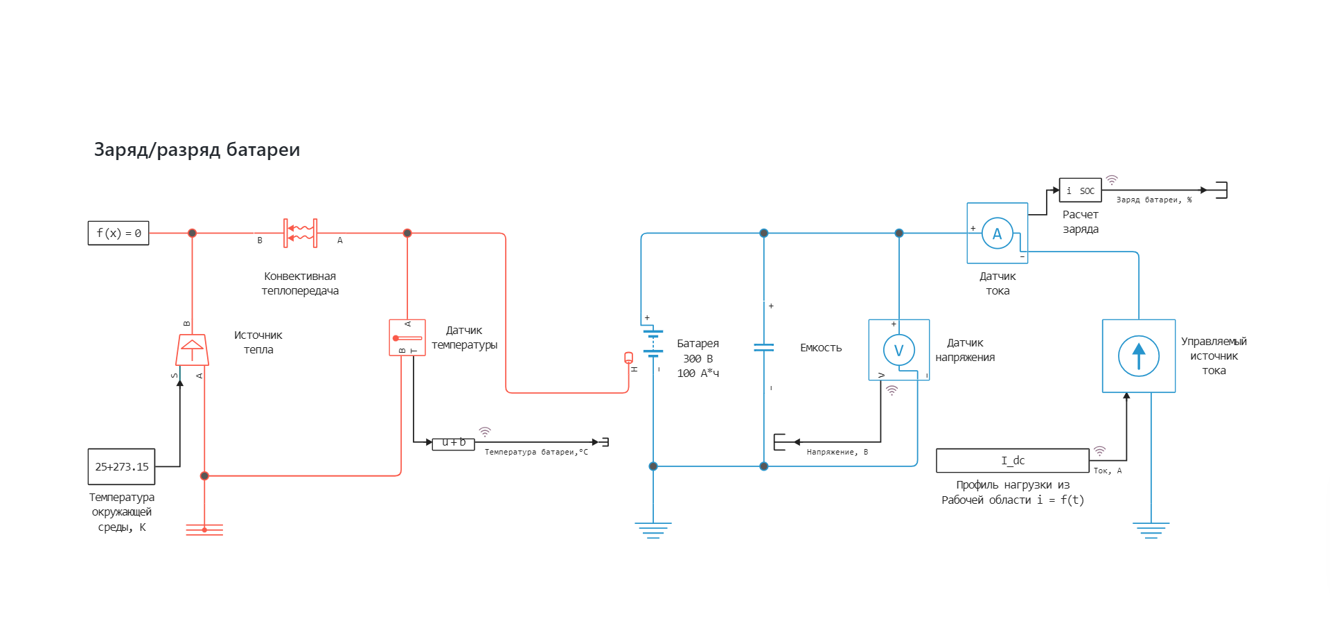
The battery is connected to a realistic DC link load profile, which is simulated using the From Workspace unit (https://engee.com/helpcenter/stable/base-lib-sources/from-workspace.html ). This unit transmits a load graph to the model in the form of a signal i = f(t) to a controlled current source.
Implementation of the model launch using software control:
Downloading the necessary libraries for importing current versus time dependence:
Pkg.add(["MAT"])
using DataFrames
using MAT
gr()
Reading a mat file and converting it to a WorkspaceArray for use in the From Workspace block:
vars = matread("/user/start/examples/power_systems/HV_battery/I_dc_discharge.mat");
data = vars["array"];
t = data[:,1];
current = data[:,2];
df = DataFrame(time=t, value=current);
I_dc = WorkspaceArray(string(rand()), df);
Loading the model:
model_name = "HV_battery"
model_name in [m.name for m in engee.get_all_models()] ? engee.open(model_name) : engee.load( "$(@__DIR__)/$(model_name).engee");
Launching the uploaded model:
results = engee.run(model_name)
Simulation results
Importing simulation results:
simulation_time = results["Voltage, V"].time;
i = results["Current, A"].value;
v = results["Voltage, V"].value;
temperature = results["Battery temperature,°C"].value;
charge = results["Battery charge, %"].value;
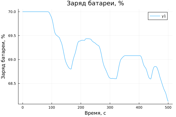
Battery charge for a time interval from 0 to 500 seconds:
plot(simulation_time[1:50000], charge[1:50000])
plot!(title = "Battery charge, %", ylabel = "Battery charge, %", xlabel="Time, c")
Load current at a time interval from 0 to 500 seconds:
plot(simulation_time[1:50000], i[1:50000])
plot!(title = "Current, A", ylabel = "Current, A", xlabel="Time, c")
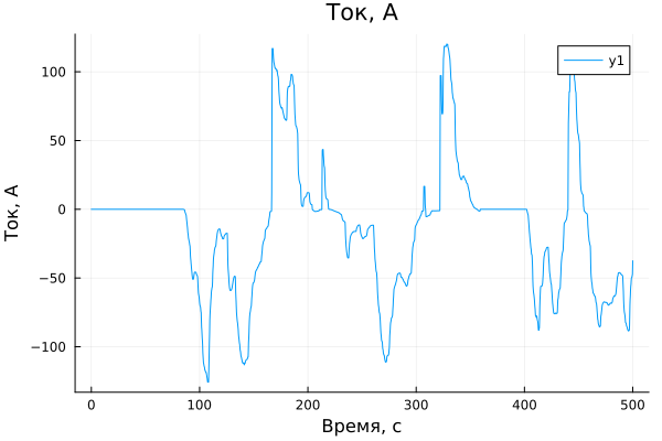
During the simulation, the battery is not only discharged, but also charged if the load current is in the opposite direction. This behavior occurs during the operation of the SNE when smoothing load fluctuations or during acceleration and braking of an electric vehicle.
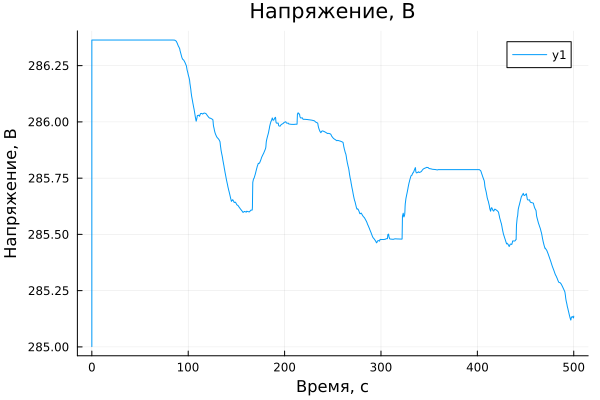
Battery voltage for a time interval from 0 to 500 seconds:
plot(simulation_time[1:50000], v[1:50000])
plot!(title = "Voltage, V", ylabel = "Voltage, V", xlabel="Time, c")
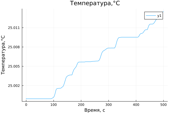
Battery temperature for a time interval from 0 to 500 seconds:
plot(simulation_time[1:50000], temperature[1:50000])
plot!(title = "Temperature,°C", ylabel = "Temperature,°C", xlabel="Time, c")
Conclusions:
In this example, tools were used for command control of a battery model with a simulation duration of 1 hour. The battery load profile was imported into the Workspace from a mat file. The simulation results were imported into a script and visualized for a given time interval using interactive graphs from the Plots library.