Speed control of a simplified synchronous generator
This example demonstrates the behaviour of a three-phase four-wire simplified synchronous alternator when switching the load in the network at:
-
The presence of a speed controller
-
Constant torque - without speed controller
General view of the model
The model is based on the library block Simplified Synchronous Machine. A simplified synchronous generator of 2000 kVA (1600 kW considering a power factor of 0.8), 600 V, 1500 rpm is connected to an active-inductive load of 1600 kW and 400 kvar. The neutral point of the machine stator winding is grounded. The internal resistance of the generator (Zg = 0.0036 + j0.16 o.u.) is the armature winding resistance Ra and the transient reactance X'd. The generator constant of inertia is H = 0.6 s, which corresponds to J = 67.5 kg*m^2.
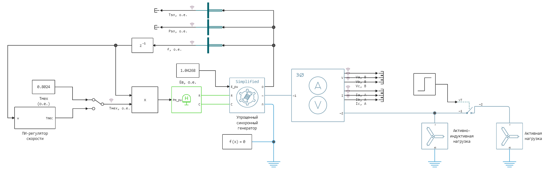
The model includes switching between constant torque Tmeh and PI speed control. Speed control is modelled using mathematical directional blocks implementing the PI controller. The synchronous machine has a constant voltage on the field winding.
A three phase circuit breaker is used to trip an 800 kW active load. The circuit breaker is initially closed and opens at time t = 1 s, which results in a 50% active load shedding.
Realisation of the model run using software control:
Loading the required libraries for importing the time dependence of the current:
using DataFrames
gr()
Running the model without speed control
Make sure that the Manual Switch is in the position to receive the signal from the Constant - Tmeh unit. The model is already in this position by default.
Load the model:
model_name = "simplified_synchronous_machine_speed_regulation"
model_name in [m.name for m in engee.get_all_models()] ? engee.open(model_name) : engee.load( "$(@__DIR__)/$(model_name).engee");
Running a loaded model:
results = engee.run(model_name)
Modelling results
Import the results of the simulation:
simulation_time = results["Ia, А"].time;
ia = results["Ia, А"].value;
ib = results["Ia, А"].value;
ic = results["Ia, А"].value;
f = results["f, о.е."].value;
Pel = results["Pэл, о.е."].value;
Tel = results["Tэл, о.е."].value;
Tmec = results["Тмех, о.е."].value;
Drawing results:
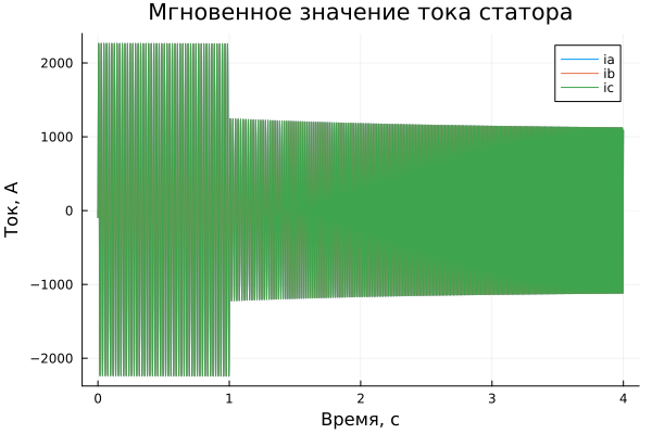
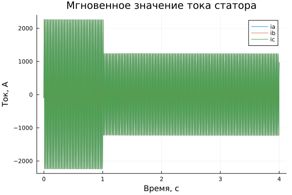
plot(simulation_time ,ia, legend=true, label="ia")
plot!(simulation_time ,ib, legend=true, label="ib")
plot!(simulation_time ,ic, legend=true, label="ic")
plot!(title = "Мгновенное значение тока статора", ylabel = "Ток, А", xlabel="Время, c")
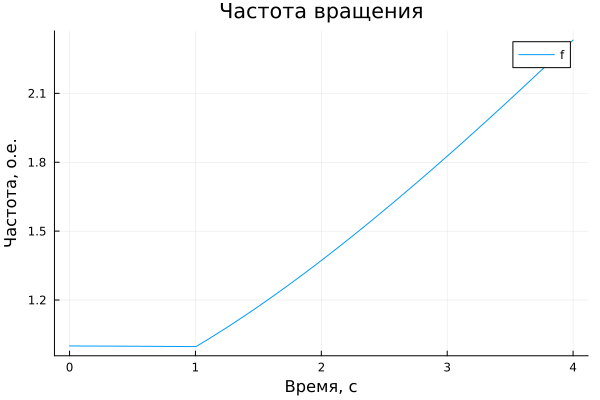
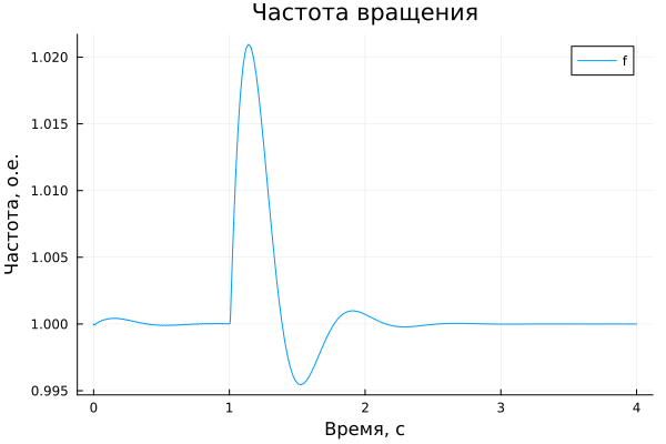
plot(simulation_time ,f, legend=true, label="f")
plot!(title = "Частота вращения", ylabel = "Частота, о.е.", xlabel="Время, c")
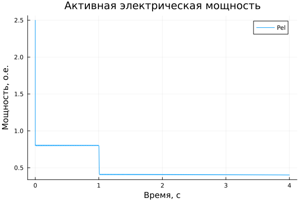
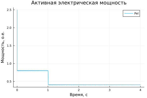
plot(simulation_time ,Pel, legend=true, label="Pel")
plot!(title = "Активная электрическая мощность", ylabel = "Мощность, о.е.", xlabel="Время, c")
plot(simulation_time ,Tel, legend=true, label="Электрический момент")
plot!(simulation_time ,Tmec, legend=true, label="Механический момент")
plot!(title = "Моменты машины", ylabel = "Момент, о.е.", xlabel="Время, c")
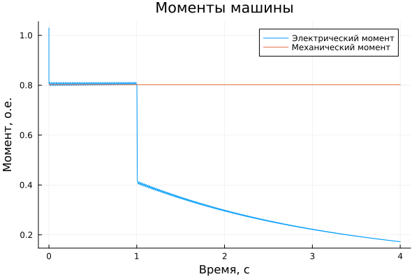
Notice when the switch opens, the electrical power drops from 0.8 o.u. to 0.4 o.u. and the machine starts to accelerate. Since the net electromechanical torque is now equal to:
The increase in speed is equal to:
One second after commutation at t = 2 s, the expected increase in speed is 0.33 o.u. In fact, the speed measured at t = 2 s is slightly higher than the theoretical value (1.374 o.u. compared to the expected 1.33 o.u.) because the electrical torque decreases as the speed increases, resulting in an electromechanical torque above 0.4 o.u.
Running the model with speed control
Now double-click on the Manual Switch block to put the speed controller into operation.
Start the model:
results = engee.run(model_name)
Modelling results
Import the results of the simulation:
simulation_time = results["Ia, А"].time;
ia = results["Ia, А"].value;
ib = results["Ia, А"].value;
ic = results["Ia, А"].value;
f = results["f, о.е."].value;
Pel = results["Pэл, о.е."].value;
Tel = results["Tэл, о.е."].value;
Tmec = results["Тмех, о.е."].value;
Drawing results:
plot(simulation_time ,ia, legend=true, label="ia")
plot!(simulation_time ,ib, legend=true, label="ib")
plot!(simulation_time ,ic, legend=true, label="ic")
plot!(title = "Мгновенное значение тока статора", ylabel = "Ток, А", xlabel="Время, c")
plot(simulation_time ,f, legend=true, label="f")
plot!(title = "Частота вращения", ylabel = "Частота, о.е.", xlabel="Время, c")
plot(simulation_time ,Pel, legend=true, label="Pel")
plot!(title = "Активная электрическая мощность", ylabel = "Мощность, о.е.", xlabel="Время, c")
plot(simulation_time ,Tel, legend=true, label="Электрический момент")
plot!(simulation_time ,Tmec, legend=true, label="Механический момент")
plot!(title = "Моменты машины", ylabel = "Момент, о.е.", xlabel="Время, c")
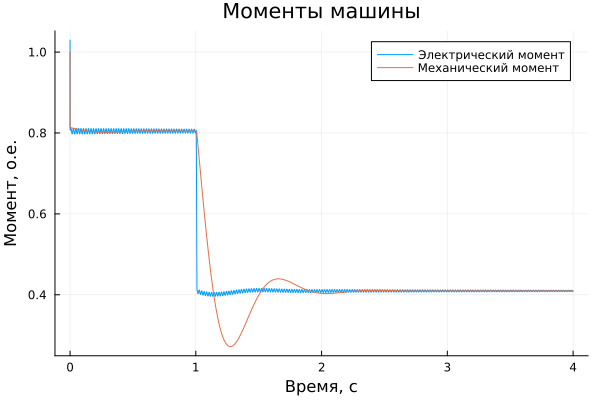
Note that the controller reduced the mechanical torque to 0.4 o.u. to maintain the speed at its reference value (1 o.u.).
Conclusions:
This example showed the operation of a simplified synchronous machine block under perturbation with and without rotational speed control. Tools for command control of the model were used, and the simulation results were imported into a script and visualised using Plots library plots.