Single-pole generator with regulators
Description of the model
This example examines the operation of a hydrogenerator-transformer unit via a double-circuit overhead line (overhead line) to an infinite-power bus with ARV-M high-power excitation regulators, rotation speed and a hydraulic turbine. At a time of 5 s. in the model, a three-phase short circuit (short circuit) occurs in the middle of one of the overhead line circuits. The model is first started with the ARV-M switched off, then the voltage control channels and its first derivative and the frequency deviation stabilization channels, its first derivative and the first derivative of the excitation current are switched on sequentially.
The process of launching and configuring the model from the script development environment using command control, processing simulation results, visualization of simulation results, and scenarios for independent work with the model are proposed. The signals are logged and their time schedules are shown. The model's appearance:
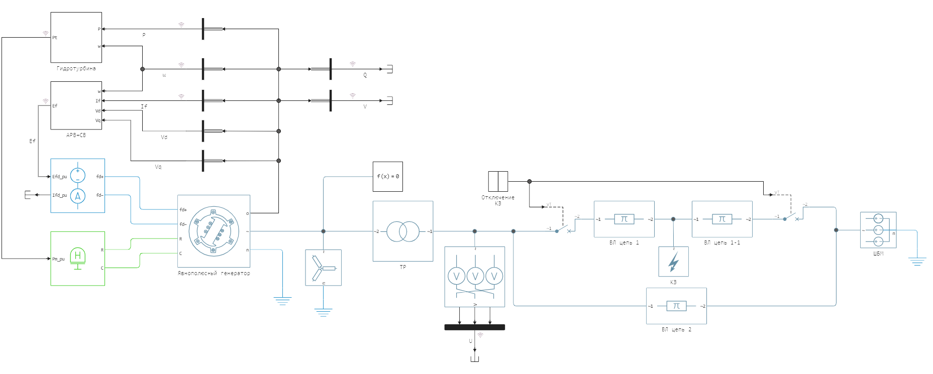
The main blocks used in this example are:
- Synchronous Machine Salient Pole - single-pole synchronous generator (, , ).
- PID-controller AVR - ARV-M excitation regulator with proportional-integral-differential voltage control law of the generator.
- Separately-Excited Exciter - an electric machine or thyristor exciter with independent power supply.
- Hydraulic Turbine and Governor - hydraulic turbine, PID control system and servo drive.
- Voltage Source (Three-Phase) - a three-phase voltage source, used to simulate the BWM, the steady-state mode is set by setting the current line voltage and phase shift (, ).
- Fault (Three-Phase) - short circuit.
- From библиотеки пассивных элементов Three-phase transmission line units Three-Phase PI Section Line (, AC 500/64, 2 circuits) and a two-winding three-phase transformer Two-Winding Transformer (Three-Phase) (TD-630000/500).
Simulation
Importing the necessary modules for working with graphs:
using Plots;
gr();
Loading the model:
model_name = "regulated_hydro_generator";
model_name in [m.name for m in engee.get_all_models()] ? engee.open(model_name) : engee.load( "$(@__DIR__)/$(model_name).engee");
Configuring the model using command control, disabling ARV:
# disabling ARV
engee.set_param!(model_name*"/АРВ+СВ/"*"reg", "Value" => 0);
# disabling the stabilization channels
engee.set_param!(model_name*"/АРВ+СВ/"*"stab", "Value" => 0);
Launching the uploaded model:
results = engee.run(model_name);
To import the simulation results, logging of the necessary signals was enabled in advance and their names were set. Converting the simulation results from the results variable:
# simulation time vector
sim_time = results["V"].time;
# vectors of recorded signals
w1 = results["w"].value;
U1 = results["V"].value;
P1 = results["P"].value;
Starting the model and turning on the ARV with only a voltage regulation channel and the first derivative without stabilization channels:
# configuring the model
engee.set_param!(model_name*"/АРВ+СВ/"*"reg", "Value" => 1);
engee.set_param!(model_name*"/АРВ+СВ/"*"stab", "Value" => 0);
# launching the model
results = engee.run(model_name);
# current vectors at measurement point No. 1
w2 = results["w"].value;
U2 = results["V"].value;
P2 = results["P"].value;
Launching the model and turning on the ARV with all channels of regulation and stabilization:
# configuring the model
engee.set_param!(model_name*"/АРВ+СВ/"*"reg", "Value" => 1);
engee.set_param!(model_name*"/АРВ+СВ/"*"stab", "Value" => 1);
# launching the model
results = engee.run(model_name);
# current vectors at measurement point No. 1
w3 = results["w"].value;
U3 = results["V"].value;
P3 = results["P"].value;
Graph of the rotation speed of the generator rotor:
plot(sim_time, w1, title = L"The speed of rotation of the rotor", ylabel = L"\omega, O.E.", xlabel=L"Time,\; c", label = L"Without \; ARV", legendfontsize = 10)
plot!(sim_time, w2, label = L"ARV\; without\; stabilization", size = (700,440), left_margin=5Plots.mm, bottom_margin=5Plots.mm)
plot!(sim_time, w3, label = L"ARV\; with\; stabilization", ylims = (0.99,1.015), legend=:topleft)
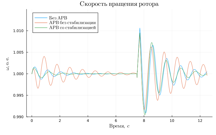
The graph shows that the use of ARV-M significantly accelerated the damping of oscillation of the generator rotor after a disturbance.
Voltage graph on generator tires:
plot(sim_time, U1, title = L"Voltage of the generator", ylabel = L"U, O.E.", xlabel=L"Time,\; c", label = L"Without \; ARV", legendfontsize = 10)
plot!(sim_time, U2, label = L"ARV\; without\; stabilization", legend=:bottomleft,size = (700,440), left_margin=5Plots.mm, bottom_margin=5Plots.mm)
plot!(sim_time, U3, label = L"ARV\; with\; stabilization", ylims = (0.3, 1.1))
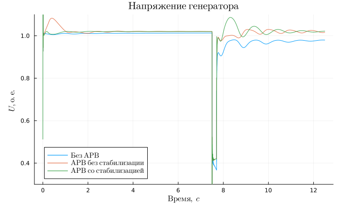
The graph shows that the use of ARV-M made it possible to restore the voltage on the generator busbars after the disturbance to the initial value.
Active power graph of the generator:
plot(sim_time, P1, title = L"Active\; generator power\;", ylabel = L"P, O.E.", xlabel=L"Time,\; c",label = L"Without \; ARV")
plot!(sim_time, P2, label = L"ARV\; without\; stabilization", legendfontsize = 10, size = (700,440), left_margin=5Plots.mm, bottom_margin=5Plots.mm)
plot!(sim_time, P3, label = L"ARV\; with\; stabilization", ylims = (0, 1.4), legend=:topleft)
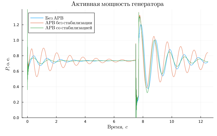
The graph shows that the use of ARV-M has significantly improved the damping of fluctuations in the active power of the generator after a disturbance.
Addition
Try to change the following model parameters yourself and explore how this affects dynamic stability:
- increase overhead line length by 200 km;
- Type of fault in the Fault (Three-Phase) block;
- Change the ARV coefficients.
Conclusions
In this example, tools were used for command management of the Engee model and uploading simulation results, and work with the Plots module is shown. The operation of a single-pole generator through a transformer and a double-circuit overhead line on a SHBM, taking into account the ARV-M, a hydraulic turbine and a rotation speed regulator, was considered. The influence of ARV-M on the operation of the power system is shown.