Analysis of transients in linear electrical circuits
The purpose of the work: To conduct a study of a linear circuit containing several electric energy storage devices in the Engee program.
The content of the work:
- create a system of equations for a given electrical circuit;
- develop a program for calculating currents in circuit branches and voltage drops on capacitive elements;
- present the results of the program calculation in the form of graphical dependencies;
- create a model of an electrical circuit in Engee;
- compare the simulation results with the calculation results of the developed program.
Engee and the DifferentialEquations.jl package are used as the software used to solve the system of equations. The calculation is carried out using the ode45 method, a one-step explicit Runge-Kutta method of the 4th (5th) order.
Here is an example of calculating a linear electrical circuit.:
1. Application of the DifferentialEquations.jl package
Package [DifferentialEquations.jl](https://diffeq.sciml.ai/stable /) provides a large number of well-optimized solvers of differential equations of various types:
- ordinary differential equations
- differential algebraic equations
- stochastic differential equations
- differential equations with a delayed argument
- stochastic differential equations with a delayed argument
- differential equations with parametric uncertainty
- and others .
Pkg.add("DifferentialEquations")
using DifferentialEquations, Plots
2. Solving the differential equation
The general procedure is as follows:
1. Set the function
f(u, p, t)
f(du, u, p, t)
where u - variables, p - equation parameters, du - derivatives .
2. Define the task
prob = ODEProblem(f, u0, tspan)
prob = ODEProblem(f, u0, tspan, p)
where u0 - initial conditions, tspan - estimated time interval ()
3. Numerical solution
sol = solve(prob, alg; kwargs)
where alg - numerical algorithm, kwargs - additional arguments.
For example, for users familiar with MATLAB/Python/R, there are translations of standard library methods.:
- ode23 → BS3()
- ode45/dopri5 → DP5(), although in most cases Tsit5() is more effective
- ode23s → Rosenbrock23(), although in most cases Rodas4() is more efficient
You can read more about solvers in документации.
4. Analysis of results
sol(t)
plot(sol)
where the function is used plot the Plots.jl package. When using other graphics packages
plot(sol.t, sol')
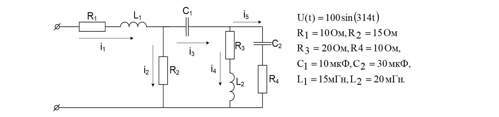
3. A program for calculating an electrical circuit
A system of differential equations describing an electrical circuit:
 where Uc1, Uc2 are the voltage across the capacitances that can be found from solving the equations

In order for the system of equations to be solvable with respect to unknown quantities standing under the sign of the differential, it is necessary to express the currents of branches that do not contain inductance in terms of the desired parameters. To do this, using Kirchhoff's laws, we formulate the coupling equations (1.2) and supplement (1.1):

# Input of electrical circuit parameters
R1 = 10.0
R2 = 15.0
R3 = 20.0
R4 = 10.0
f = 50.0
C1 = 10e-6
C2 = 30e-6
L1 = 15e-3
L2 = 20e-3
# Definition of the differential system
function circuit!(du, u, p, t)
U, R1, R2, R3, R4, C1, C2, L1, L2 = p
Uc1, Uc2, i1, i4 = u
# Algebraic communication equations
i2 = (u[1] + u[2] + (u[3] - u[4]) * R4) / (R2 + R4)
i3 = u[3] - i2
i5 = i3 - u[4]
# Differential equations
du[1] = i3 / C1
du[2] = i5 / C2
du[3] = 1 / L1 * (U(t) - i2 * R2 - u[3] * R1)
du[4] = 1 / L2 * (u[2] + i5 * R4 - u[4] * R3)
end
# Initial conditions for u
u0 = [0.0, 0.0 , 0.0, 0.0]
# The time range for calculation, let there be two periods of the industrial frequency of 50 Hz
tspan = (0.0, 0.04)
# Setting parameters
U(t) = 100 * sin(2 * π * f * t)
params = (U, R1, R2, R3, R4, C1, C2, L1, L2)
# Creating an ODEProblem object with passing parameters
prob = ODEProblem(circuit!, u0, tspan, params)
# Solving differential equations
sol = solve(prob, Tsit5());
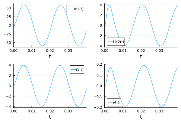
# Plotting graphs
plot(sol, label = ["Uc1(t)" "Uc2(t)" "i1(t)" "i4(t)"], layout = 4)
4. Comparison of calculation results with simulation results
Let's load the model located in /user/start/examples/power_systems/lab_work/lab_work.engee.
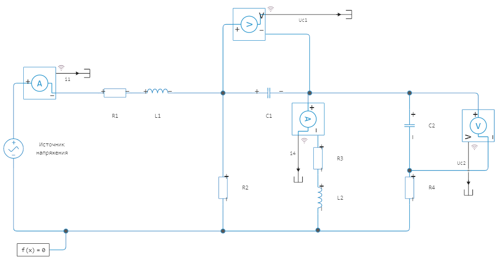
modelName = "lab_work";
model = modelName in [m.name for m in engee.get_all_models()] ? engee.open( modelName ) : engee.load( "$(@__DIR__)/$(modelName).engee");
Let's run the simulation:
results = engee.run( modelName );
Let's give convenient names to the output variables of our model (those that are marked as logged signals):
t = results["i1"].time;
i1 = results["i1"].value;
i4 = results["i4"].value;
Uc1 = results["Uc1"].value;
Uc2 = results["Uc2"].value;
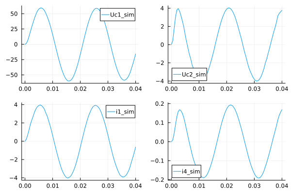
Let's build graphs based on the simulation results.:
plot(t, [Uc1 Uc2 i1 i4], label = ["Uc1_sim" "Uc2_sim" "i1_sim" "i4_sim"], layout = 4)
Let's display the simulation results and calculation results on one graph.:
plot(t, [Uc1 Uc2 i1 i4], label = ["Uc1_sim" "Uc2_sim" "i1_sim" "i4_sim"], layout = 4)
plot!(sol, label = ["Uc1" "Uc2" "i1" "i4"], layout = 4)
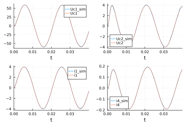
Conclusions on the work: in the course of the work, a system of algebraic differential equations was compiled, a program for calculating currents in branches and voltage drops on capacitive circuit elements was developed, graphical dependences of the laws of current and voltage variation on time are shown. The results of Engee modeling are compared with the results of the developed calculation program. In general, the laboratory work presents an analysis of an electrical circuit containing several electric energy storage devices.