Short circuits on power lines in a network with a grounded neutral
Description of the model
This example considers a power system with a dead-earthed neutral consisting of two overhead lines with two-way power supply and one dead-end line at the end of which a short circuit (short circuit) occurs followed by disconnection (by default, the model has a single-phase short circuit to ground in phase A). The process of launching a model from the script development environment using command control, processing simulation results, calculating symmetric components, visualizing simulation results, and offering scenarios for independent work with the model are shown. The values of currents and voltages are logged at three measurement points, their time graphs and vector diagrams are shown, and the Fortescue transform is performed to calculate the symmetrical components. The model's appearance:
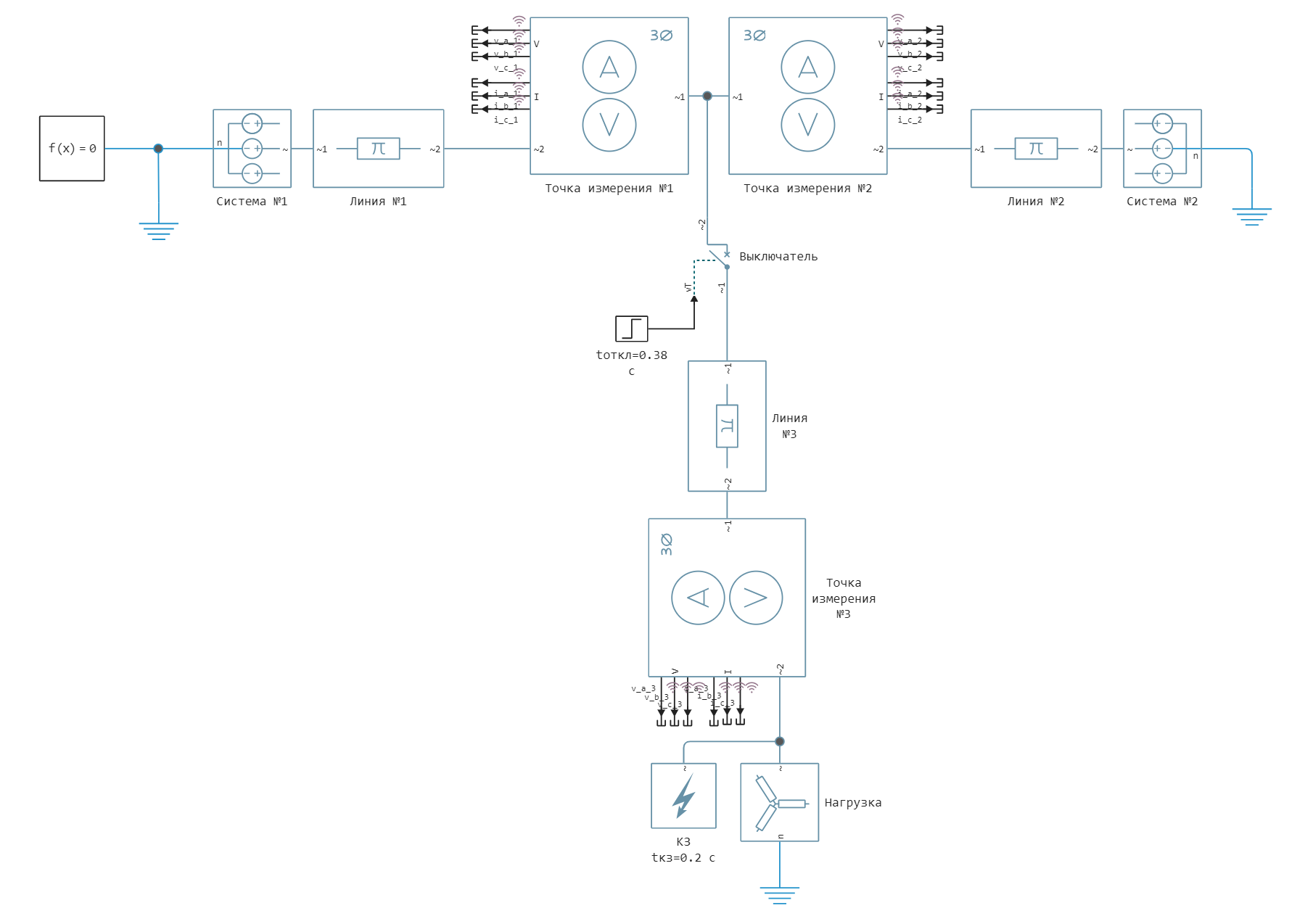
The systems are modeled in blocks Voltage Source (Three-Phase), the steady-state mode is set by setting the current line voltage and phase shift. Overhead lines are modeled by blocks Three-Phase PI Section Line. A short circuit is modeled by a block Fault (Three-Phase) in the settings of this block, using the Failure mode drop-down menu, you can select the type of short circuit. The short circuit is disabled using the block Circuit Breaker (Three-Phase), which simulates the operation of relay protection. The duration of the short-circuit shutdown is selected based on the operating time of the dead-end line protections with one-way power supply and the switch-off time, and is set to 0.18 s at the upper limit of the short-circuit shutdown duration for 110 kV in accordance with the Methodological Guidelines on the Stability of Power Systems from 2003 [1]. The load is modeled by the block Wye-Connected Load.
System parameters [2]:
| Element | Parameter |
|---|---|
| System No. 1 | Balancing node |
| System No. 2 | |
| Load | |
| Line No. 1 | AC 185/29 |
| Line No. 2 | AC 185/29 |
| Line No. 3 | AC 150/24 |
Launching the model
We will import the necessary modules for working with graphs, tables, and a floating-window Fourier transform function.:
using Plots
using DataFrames
include("$(@__DIR__)/fourie_func.jl")
gr();
Loading the model:
model_name = "grounded_neutral_network_fault"
model_name in [m.name for m in engee.get_all_models()] ? engee.open(model_name) : engee.load( "$(@__DIR__)/$(model_name).engee");
Launching the uploaded model:
results = engee.run(model_name);
Simulation results
To import the simulation results, logging of the necessary signals was enabled in advance and their names were set. We convert the instantaneous values of currents and voltages of the results variable into separate vectors:
# simulation time vector
sim_time = results["i_a_1"].time;
# vector of currents at the measuring point No. 1
i_1 = hcat(results["i_a_1"].value,results["i_b_1"].value,results["i_c_1"].value);
# vector of currents at the measuring point No. 2
i_2 = hcat(results["i_a_2"].value,results["i_b_2"].value,results["i_c_2"].value);
# vector of currents at the measuring point No. 3
i_3 = hcat(results["i_a_3"].value,results["i_b_3"].value,results["i_c_3"].value);
# stress vector at the measuring point No. 1
v_1 = hcat(results["v_a_1"].value,results["v_b_1"].value,results["v_c_1"].value);
# stress vector at the measuring point No. 2
v_2 = hcat(results["v_a_2"].value,results["v_b_2"].value,results["v_c_2"].value);
# stress vector at the measuring point No. 3
v_3 = hcat(results["v_a_3"].value,results["v_b_3"].value,results["v_c_3"].value);
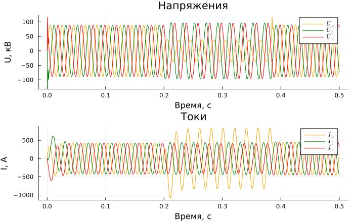
Graphs of currents and voltages at the measuring point No. 1:
p1 = Plots.plot(sim_time, v_1./1e3, label = [L"U_a" L"U_b" L"U_c"],
title = "Voltage", ylabel = "U, kV", xlabel="Time, c");
p2 = Plots.plot(sim_time, i_1, label = [L"I_a" L"I_b" L"I_c"],
title = "Currents", ylabel = "I, And", xlabel="Time, c")
plot(p1, p2, layout=(2,1), legend = true, linecolor = [:orange :green :red], size = (700,440))

Graphs of currents and voltages at the measuring point No. 2:
p1 = Plots.plot(sim_time, v_2./1e3, label = [L"U_a" L"U_b" L"U_c"],
title = "Voltage", ylabel = "U, kV", xlabel="Time, c");
p2 = Plots.plot(sim_time, i_2, label = [L"I_a" L"I_b" L"I_c"],
title = "Currents", ylabel = "I, And", xlabel="Time, c")
plot(p1, p2, layout=(2,1), legend = true, linecolor = [:orange :green :red], size = (700,440))
Graphs of currents and voltages at the measuring point No. 3
p1 = Plots.plot(sim_time, v_3./1e3, label = [L"U_a" L"U_b" L"U_c"],
title = "Voltage", ylabel = "U, kV", xlabel="Time, c");
p2 = Plots.plot(sim_time, i_3, label = [L"I_a" L"I_b" L"I_c"],
title = "Currents", ylabel = "I, And", xlabel="Time, c")
plot(p1, p2, layout=(2,1),legend = true, linecolor = [:orange :green :red], size = (700,440))
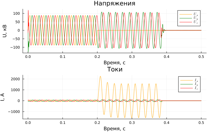
As a result of a single-phase short circuit, the voltage of the damaged phase decreases and the current increases. Note that the voltage of the damaged phase increases as you move away from the damage site.
Processing of results
Let's evaluate the effect of short-circuit on the asymmetry of currents. Calculation of symmetric components using the Fortescue transform [3]:
To do this, we perform vectorization of the currents using a Fourier transform with a floating window to isolate the amplitudes and phases.
At the same time, we will not use the built-in functions and will use the function [4]:
# Variables for storing vectors
v_1_Xmag, v_2_Xmag, v_3_Xmag, i_1_Xmag, i_2_Xmag, i_3_Xmag,
v_1_Xphase, v_2_Xphase, v_3_Xphase, i_1_Xphase, i_2_Xphase, i_3_Xphase = [zeros(length(sim_time),3) for _ = 1:12];

for (Xmag, Xphase, signal) in zip(
    (v_1_Xmag, v_2_Xmag, v_3_Xmag, i_1_Xmag, i_2_Xmag, i_3_Xmag),
    (v_1_Xphase, v_2_Xphase, v_3_Xphase, i_1_Xphase, i_2_Xphase, i_3_Xphase),
    (v_1, v_2, v_3, i_1, i_2, i_3))
    Xmag, Xphase = moving_fourie(Xmag, Xphase, sim_time, signal);
end
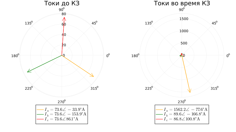
Vector diagram of currents at measuring point No. 3 before and during short circuit:
# search for indices of moments before and after the short circuit (0.1 s and 0.3 s)
nom_reg_ind = indexin(0.1, sim_time);
kz_ind = indexin(0.3, sim_time);
# current amplitudes and phases
i_a_NR_mag, i_a_NR_ang = round(i_3_Xmag[nom_reg_ind,1][1], digits=1), round(i_3_Xphase[nom_reg_ind,1][1], digits=1)
i_b_NR_mag, i_b_NR_ang = round(i_3_Xmag[nom_reg_ind,2][1], digits=1), round(i_3_Xphase[nom_reg_ind,2][1], digits=1)
i_c_NR_mag, i_c_NR_ang = round(i_3_Xmag[nom_reg_ind,3][1], digits=1), round(i_3_Xphase[nom_reg_ind,3][1], digits=1)
i_a_SC_mag, i_a_SC_ang = round(i_3_Xmag[kz_ind,1][1], digits=1), round(i_3_Xphase[kz_ind,1][1], digits=1)
i_b_SC_mag, i_b_SC_ang = round(i_3_Xmag[kz_ind,2][1], digits=1), round(i_3_Xphase[kz_ind,2][1], digits=1)
i_c_SC_mag, i_c_SC_ang = round(i_3_Xmag[kz_ind,3][1], digits=1), round(i_3_Xphase[kz_ind,3][1], digits=1)

p1 = plot([0;i_a_NR_ang*pi/180], [0;i_a_NR_mag], arrow=true, proj = :polar, linecolor = :orange,
label = L"I_a = %$i_a_NR_mag \angle\, %$i_a_NR_ang\degree And", title = "Currents up to short circuit")

plot!([0;i_b_NR_ang*pi/180], [0;i_b_NR_mag], arrow=true, proj = :polar, linecolor = :green,
label = L"I_b = %$i_b_NR_mag \angle\, %$i_b_NR_ang \degree And")

plot!([0;i_c_NR_ang*pi/180], [0;i_c_NR_mag], arrow=true, proj = :polar, linecolor = :red,
label = L"I_c = %$i_c_NR_mag \angle\, %$i_c_NR_ang\degree And")

p2 = plot([0;i_a_SC_ang*pi/180], [0;i_a_SC_mag], arrow=true, proj = :polar, linecolor = :orange,
label = L"I_a = %$i_a_SC_mag \angle\, %$i_a_SC_ang \degree And", title = "Currents during short circuit")

plot!([0;i_b_SC_ang*pi/180], [0;i_b_SC_mag], arrow=true, proj = :polar, linecolor = :green,
label = L"I_b = %$i_b_SC_mag \angle\, %$i_b_SC_ang \degree And")

plot!([0;i_c_SC_ang*pi/180], [0;i_c_SC_mag], arrow=true, proj = :polar, linecolor = :red,
label = L"I_c = %$i_c_SC_mag \angle\, %$i_c_SC_ang\degree And")

plot(p1, p2, layout=(1,2), legend = :outerbottom, legendfontsize=10, size = (800,450))
Consider the current distribution of phase A at the junction of line No. 1-3 during a short circuit in a vector diagram:
# vectors of currents in complex numbers
i_a_1_mag, i_a_1_ang = round(i_1_Xmag[kz_ind,1][1], digits=1), round(i_1_Xphase[kz_ind,1][1], digits=1)
i_a_2_mag, i_a_2_ang = round(i_2_Xmag[kz_ind,1][1], digits=1), round(i_2_Xphase[kz_ind,1][1], digits=1)
i_a_3_mag, i_a_3_ang = round(i_3_Xmag[kz_ind,1][1], digits=1), round(i_3_Xphase[kz_ind,1][1], digits=1)
ia1 = i_a_1_mag*exp(1im*i_a_1_ang*pi/180)
ia2 = i_a_2_mag*exp(1im*i_a_2_ang*pi/180)
ia3 = i_a_3_mag*exp(1im*i_a_3_ang*pi/180)

plot([0;angle(ia1)], [0;abs(ia1)],
 arrow=true, proj = :polar, linecolor = :orange, label =  L"I_{a1} = %$i_a_1_mag \angle\, %$i_a_1_ang \degree")

plot!([0;angle(ia2)], [0;abs(ia1)],
 arrow=true, proj = :polar, linecolor = :green, label = L"I_{a2} = %$i_a_2_mag \angle\, %$i_a_2_ang \degree And")

plot!([0;angle(ia3)], [0;abs(ia3)],
 arrow=true, proj = :polar, linecolor = :red, label = L"I_{a3} = %$i_a_3_mag \angle\, %$i_a_3_ang \degree And")

# auxiliary vector Ia3+Ia1
plot!([angle(ia3);angle(ia3+ia1)], [abs(ia3);abs(ia3+ia1)],
 arrow=true, proj = :polar, linecolor = :orange, label = L"I'_{a1} = %$i_a_1_mag \angle\, %$i_a_1_ang\degree",
  ls = :dash, linewidth=0.3)

# auxiliary vector Ia3+Ia1+Ia2
plot!([angle(ia3+ia1);angle(ia3+ia1+ia2)], [abs(ia3+ia1);abs(ia3+ia1+ia2)], arrow=true, proj = :polar, linecolor = :green,
label = L"I'_{a2} = %$i_a_2_mag \angle\, %$i_a_2_ang \degree And", ls = :dash, linewidth=0.3, legendfontsize=10, legend = :outerbottom)
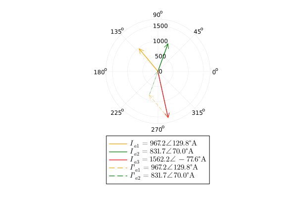
The vector diagram shows that the geometric sum of the currents is and is equal to the current , and all the currents add up to 0. This diagram shows the fulfillment of Kirchhoff's first law for a node.
Calculate the symmetrical components of the currents:
a = exp(2pi*1im/3)
a_matr = [1 1 1;
         a a^2 1;
         a^2 a 1;]
# Symmetric components: [I1 I2 I0]
i_3_sym = 1/3*(i_3_Xmag .* exp.(1im .* i_3_Xphase .* (pi/180)))*a_matr;
Let's tabulate the values of the amplitudes and symmetrical components of the currents (measuring point No. 3) before and during the short circuit.:
# Currents No. 3
println("\n"*"Currents at the measuring point No. 3")
println(DataFrame([["Nom.dir.", "KZ"],
round.([i_3_Xmag[nom_reg_ind,1][1]; i_3_Xmag[kz_ind,1][1]],digits = 1),
round.([i_3_Xmag[nom_reg_ind,2][1]; i_3_Xmag[kz_ind,2][1]],digits = 1),
round.([i_3_Xmag[nom_reg_ind,3][1]; i_3_Xmag[kz_ind,3][1]],digits = 1),
round.(abs.([i_3_sym[nom_reg_ind,1][1]; i_3_sym[kz_ind,1][1]]),digits = 1),
round.(abs.([i_3_sym[nom_reg_ind,2][1]; i_3_sym[kz_ind,2][1]]),digits = 1),
round.(abs.([i_3_sym[nom_reg_ind,3][1]; i_3_sym[kz_ind,3][1]]),digits = 1)],
["Modes", "I_a (A)", "I_b (A)", "I_c (A)", "I_1 (A)", "I_2 (A)", "I_0 (A)"]))
With a single-phase short circuit to earth, the components of the reverse and zero sequences appear, and they are practically equal to each other. The small difference in values is due to the presence of a load at the end of line No. 3.
Addition
Try to change the following model parameters yourself and investigate how this affects the operating mode of the power system:
- the length of line No. 3 is 60 km;
- Type of fault in the Fault (Three-Phase) block;
- The value of the short-circuit transition resistance at 0.1 ohms in the Fault (Three-Phase) block;
- 3-phase short circuit power for 3000 MVA power supplies - Voltage Source (Three-Phase) units.
Conclusions
In this example, tools were used for command management of the Engee model and uploading simulation results, and work with the Plots and DataFrames modules is shown. The measured currents and voltages were imported into the Workspace from the result variable and then displayed on time graphs. They were then vectorized using a Fourier transform with a floating window and shown on vector diagrams. Based on the obtained vectors of currents and voltages using the Fortescue transform, the symmetric components are calculated and tabulated.
Links
- Methodological guidelines on the stability of energy systems.
Approved by the Order of the Ministry of Energy of Russia dated June 30, 2003 N 277. - Handbook on the design of electrical networks /
edited by D. L. Faybisovich. – 4th ed., revised and add. – M. : ENAS, 2012. – 376 p. : ill. - Zeveke G.V., Ionkin P.A., Netushil A.V., Strakhov S.V. Fundamentals of circuit theory (4th ed., 1975).
- Microprocessor relays : a textbook / A. A. Nikitin ; Ministry of Education and Science of the Russian Federation, Federal Agency for Education, Federal State Educational Institution higher Prof. education "Chuvash State University named after I. N. Ulyanov". Cheboksary : Publishing House of the Chuvash University, 2006. 447 p.; ISBN 5-7677-1051-1