Overhead line closure with mutual induction
Description of the model
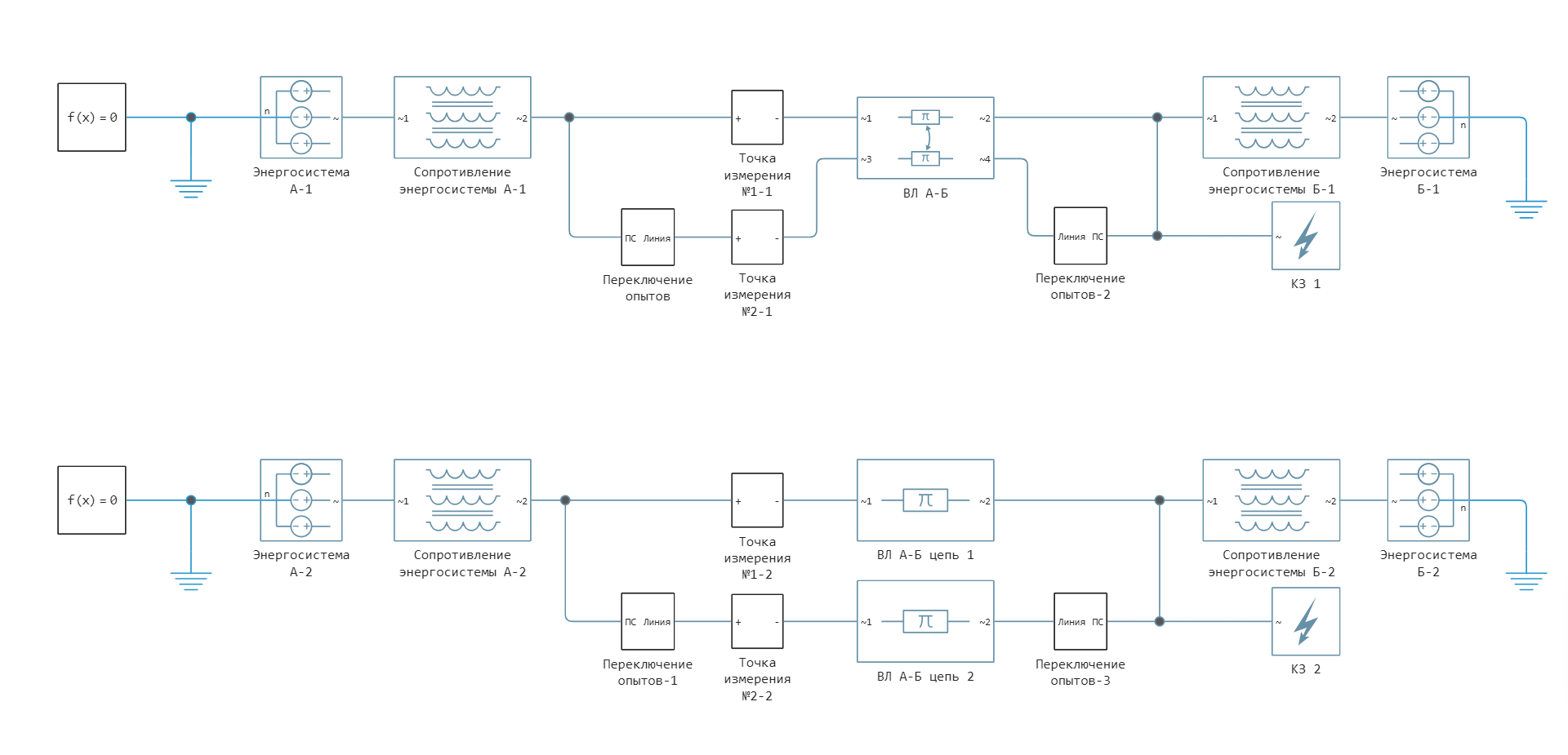
In this example, two independent 220 kV power systems with a dead-earth neutral are considered, consisting of two-circuit overhead lines (overhead lines) with two-way power supply from substations (PS) A and PS B. In the first overhead line power system, it is modeled by a block Double-Circuit Transmission Line, which is a U-shaped substitution scheme taking into account the mutual induction between the chains. In the second power grid, the overhead line is modeled by a block Three-Phase PI Section Line, which is a conventional U-shaped substitution scheme.
The mutual induction between overhead line circuits can significantly affect the calculation results of some asymmetric modes. For example, when calculating the settings of the first stage of the zero-sequence directional current protection
(TNNR), one of the conditions for detuning from the tripled zero-sequence current (NP) passing at the protection installation site is [1]:
- in case of an earth fault on the busbars of the opposite substation;
- in case of an earth fault on the busbars of the opposite substation, if the parallel circuit is disconnected and grounded at both ends and the mutual induction between the lines cannot be neglected.
Next, the above scenarios will be shown, the process of launching and configuring the model from the script development environment using command control, processing simulation results, visualizing simulation results, and scenarios for independent work with the model will be proposed. The current values are logged, and their time schedules are shown. The model is configured for each of the scenarios by changing the positions of the switches in the "Experiment Switching" subsystems. The model's appearance:
Power systems are modeled by a block Voltage Source (Three-Phase), the steady-state mode is set by setting the current line voltage and phase shift. The resistances of the direct and zero sequence of power systems are modeled by the block Coupled Lines (Three-Phase). A short circuit is modeled by a block Fault (Three-Phase) in the settings of this block, using the Failure mode drop-down menu, you can select the type of short circuit. The system parameters are set in accordance with Appendix B1 "The program of functional tests of DZ and TNZP 110-220 kV" [2]:
| Element | Parameter |
|---|---|
| System A | Equivalent EMF |
| System B | Equivalent EMF |
| Line A-B | |
The experience of an earth fault on the tires of the opposite PS
Importing the necessary modules for working with graphs:
using Plots
gr();
Loading the model:
model_name = "mutual_inductance_line";
model_name in [m.name for m in engee.get_all_models()] ? engee.open(model_name) : engee.load( "$(@__DIR__)/$(model_name).engee");
The model is configured for the first experiment with a 1-f short circuit on PS B buses with two overhead line circuits running by changing the values of the constant blocks connected to the switches in the "Experiment Switching" subsystems. If the value of the constant is zero, then the switch is in a closed state, otherwise it opens. Thus, to connect the second circuits from the PS A and PS B busbars and disconnect the grounding from both ends, the following constants must be set:
enable_step_name = "Switching Experiences/Enable";
grounding_step_name = "Switching Experiences/Grounding";
# Switching on the PS switches
engee.set_param!(model_name*"/"*enable_step_name, "Value" => 0);
# Disconnecting grounding switches
engee.set_param!(model_name*"/"*grounding_step_name, "Value" => 1);
Launching the uploaded model:
results = engee.run(model_name);
To import the simulation results, logging of the necessary signals was enabled in advance and their names were set. Converting the instantaneous values of the currents of the results variable into separate vectors:
# simulation time vector
sim_time = results["i_a_1"].time;
# current vectors at measurement point No. 1
i_1mut = hcat(results["i_a_1mut"].value,results["i_b_1mut"].value,results["i_c_1mut"].value,results["sum_i_1mut"].value);
i_1 = hcat(results["i_a_1"].value,results["i_b_1"].value,results["i_c_1"].value,results["sum_i_1"].value);
# current vectors at the measuring point No. 2
i_2mut = hcat(results["i_a_2mut"].value,results["i_b_2mut"].value,results["i_c_2mut"].value,results["sum_i_2mut"].value);
i_2 = hcat(results["i_a_2"].value,results["i_b_2"].value,results["i_c_2"].value,results["sum_i_2"].value);
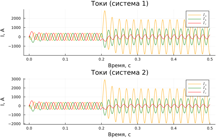
Graphs of currents at measuring point 1 (beginning of circuit 1 on side of PS A):
p1 = plot(sim_time, i_2mut[:,1:3], label = [L"I_a" L"I_b" L"I_c"],
title = "Currents (system 1)", ylabel = "I, And", xlabel="Time, c");
p2 = plot(sim_time, i_2[:,1:3], label = [L"I_a" L"I_b" L"I_c"],
title = "Currents (system 2)", ylabel = "I, And", xlabel="Time, c")
plot(p1, p2, layout=(2,1), legend = true, linecolor = [:orange :green :red], size = (700,440))
Graphs of tripled currents of the zero sequence at measurement points 1 and 2 (the beginning of the overhead line from the side of the substation):
p1 = plot(sim_time, [i_1mut[:,4] i_1[:,4]], label = [L"3I_0(system\,1)" L"3I_0(system\,2)"],
title = "Tripled NP currents at the measuring point 1", ylabel = "I, And", xlabel="Time, c")
p2 = plot(sim_time, [i_2mut[:,4] i_2[:,4]], label = [L"3I_0(system\,1)" L"3I_0(system\,2)"],
title = "Tripled NP currents at the measuring point 2", ylabel = "I, And", xlabel="Time, c")
plot(p1, p2, layout = (2,1), size = (700,440))
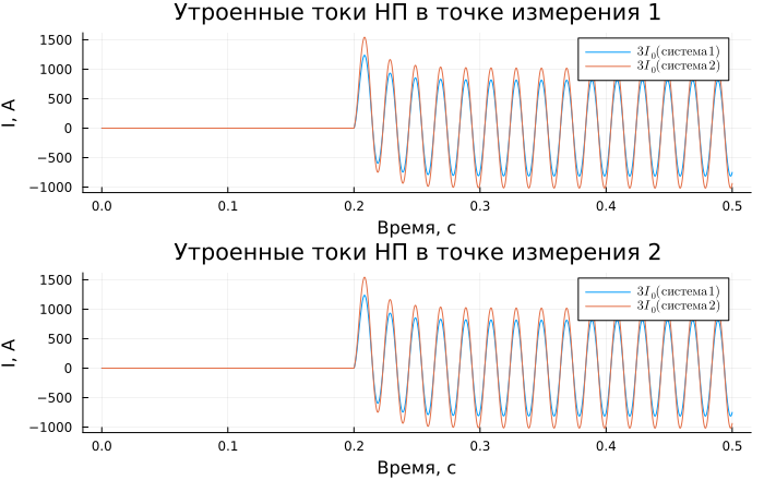
When mutual induction is taken into account, the tripled NP current becomes smaller due to an increase in the total resistance of the NP overhead line.
Experience with an earth fault on PS B busbars if the parallel circuit is disconnected and grounded at both ends:
Setting up the model for the second experiment with a short circuit on PS B tires with one circuit disconnected and grounded, by analogy with the previous experience:
# disconnecting the second circuits from the PS A and PS B busbars and grounding at both ends
enable_step_name = "Switching Experiences/Enable";
grounding_step_name = "Switching Experiences/Grounding";
# Disabling the circuit breakers
engee.set_param!(model_name*"/"*enable_step_name, "Value" => 1);
# Turning on the grounding switches
engee.set_param!(model_name*"/"*grounding_step_name, "Value" => 0);
Running the loaded model and importing the results:
results = engee.run(model_name);
# current vectors at measurement point No. 1
i_1mut = hcat(results["i_a_1mut"].value,results["i_b_1mut"].value,results["i_c_1mut"].value,results["sum_i_1mut"].value);
i_1 = hcat(results["i_a_1"].value,results["i_b_1"].value,results["i_c_1"].value,results["sum_i_1"].value);
# current vectors at the measuring point No. 2
i_2mut = hcat(results["i_a_2mut"].value,results["i_b_2mut"].value,results["i_c_2mut"].value,results["sum_i_2mut"].value);
i_2 = hcat(results["i_a_2"].value,results["i_b_2"].value,results["i_c_2"].value,results["sum_i_2"].value);
Graphs of tripled currents of the zero sequence at measurement points 1 and 2 (the beginning of the overhead line from the side of the substation):
p1 = plot(sim_time, [i_1mut[:,4] i_1[:,4]], label = [L"3I_0(system\,1)" L"3I_0(system\,2)"],
title = "Tripled NP currents at the measuring point 1", ylabel = "I, And", xlabel="Time, c")
p2 = plot(sim_time, [i_2mut[:,4] i_2[:,4]], label = [L"3I_0(system\,1)" L"3I_0(system\,2)"],
title = "Tripled NP currents at the measuring point 2", ylabel = "I, And", xlabel="Time, c")
plot(p1, p2, layout = (2,1), size = (700,440))
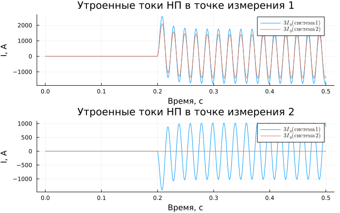
The graph shows that due to mutual induction, the first circuit induces NP currents in the second. When mutual induction is taken into account, the tripled NP current becomes larger. In this mode, the NP resistance of the two-chain overhead line is minimal. As can be seen from the experiments, taking into account the mutual induction between overhead line circuits can have a strong effect on currents, and as a result, on the calculation of protection response settings.
Addition
Try to change the following model parameters yourself and explore how this affects the simulation results:
- overhead line length by 140 km;
- Type of fault in the Fault (Three-Phase) block;
- the specific inductive resistance of mutual induction at 1 Ohm / km.
Conclusions
In this example, tools were used for command management of the Engee model and uploading simulation results, and work with the Plots module is shown. The measured currents were imported into the Workspace from the result variable and then displayed on time graphs. The use of the Double-Circuit Transmission Line block, which takes into account the mutual induction between overhead line circuits, and a comparison with a conventional overhead line block is shown.
Links
- Methodology for calculating and selecting settings (settings) and algorithms for the operation of backup protections in a cabinet type SHE2607 021. URL: https://ekra.ru/product/docs/rz-ps-110-750kv/zashchita-lin/she2607-she2710/Recommendations according to%20account%20stocks%20KX%20110-220%20kV.pdf?ysclid=m2oicx6k7852299404 (accessed 10/28/2024)
- The standard of organization of FGC UES PJSC. STO 56947007-29.120.70.241-2017. Technical requirements for microprocessor devices RPA. URL: https://www.rosseti.ru/upload/iblock/bc9/wgavy1h2g4grcll6x2rmxfltcjatlcfk.pdf (accessed 28.10.2024)