An implicit pole generator without regulators
Description of the model
This example examines the operation of a turbogenerator-transformer unit via a two-circuit overhead line (overhead line) to an infinite-power bus without regulators of excitation and rotation speed. At a time of 5 s. in the model, a three-phase short circuit (short circuit) occurs at the beginning of one of the overhead line circuits. An analytical calculation of the terminal shutdown time using the area method is carried out and compared with the results of mathematical modeling [1-3].
The process of launching and configuring the model from the script development environment using command control, processing simulation results, visualization of simulation results, and scenarios for independent work with the model are proposed. The signals are logged and their time schedules are shown. The model's appearance:
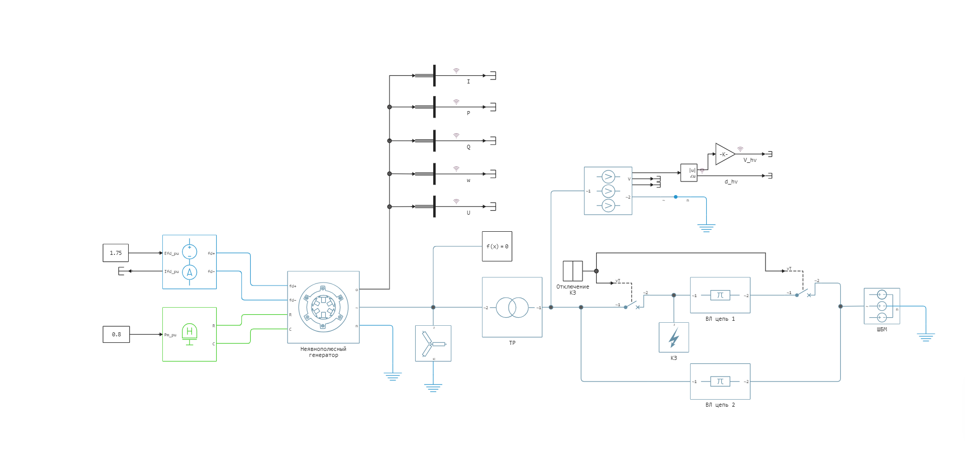
The main blocks used in this example and their parameters:
- Synchronous Machine Round Rotor - an implicit-pole synchronous generator (,).
- Voltage Source (Three-Phase) - a three-phase voltage source, used to simulate the BWM, the steady-state mode is set by setting the current line voltage and phase shift (,).
- Fault (Three-Phase) - short circuit.
- From библиотеки пассивных элементов Three-phase transmission line units Three-Phase PI Section Line (, AC 500/64, 2 circuits) and a two-winding three-phase transformer Two-Winding Transformer (Three-Phase) (TD-630000/500).
Calculation of the cut-off angle using the area method
Importing the necessary modules for working with graphs:
using Plots;
gr();
SBM Parameters:
# rated voltage, V
Us = 500e3
# short circuit power, VA
Skz = 10e9
# total resistance of the system, ohms
Zkz = Us ^ 2 / Skz
# the ratio of active and inductive resistance
XR = 15
# inductive resistance of the system, ohms
Xkz = Zkz * sin(atan(XR))
# active resistance of the system, ohms
Rkz = Zkz * cos(atan(XR))
# complex system resistance, ohms
Zs = Rkz + 1im * Xkz;
Power line parameters:
# resistivity of the direct sequence, Ohms/km
Z0 = 0.01967 + 0.2899im
# number of circuits
n = 2
# overhead line length, km
L = 200
# specific capacitive conductivity, Cm/km
b0 = 3.908e-6
bc = b0 * L * n
# total overhead line resistance, ohms
Zl = Z0 * L / n
# capacitive resistance of half overhead line, ohms
Zc = -2im / bc;
Transformer Parameters:
# active resistance TR, Ohms
Rt = 0.4514
# inductive resistance TR, ohms
Xt = 30.62
Zt = Rt + Xt * 1im;
Generator Parameters:
# rated voltage, V
Ug = 24e3
# rated power, VA
Sg = 500e6
# active resistance, O.E.
Ra = 0.003
# synchronous inductive resistance along the d axis, O.E.
Xd = 1.81
# transient inductive resistance along the d axis, O.E.
Xdd = 0.3
# complex transient resistance of the generator, ohms
Zg = (Ra + Xdd * 1im) * Us ^ 2 / Sg;
Load Parameters:
# active load power, W
Pn = 20e6
# active load resistance, ohms
Zn = Us ^ 2 / Pn;
Calculation of own and mutual resistances and in normal mode, using the single current method:
I2 = 1
Uc = I2 * Zs
Ic0 = Uc / Zc
Ibc = I2 + Ic0
Ub = Uc + Zl * Ibc
Ib0 = Ub / Zc
Iab = Ib0 + Ibc
Ua = Ub + Iab * Zt
Ia0 = Ua / Zn
I1 = Ia0 + Iab
U1 = Ua + I1 * (Xdd * 1im * Us ^ 2 / Sg)
Z12d = (Ua + I1 * (Xd * 1im * Us ^ 2 / Sg)) / I2
Z12 = U1 / I2
Z11 = U1 / I1
alpha11 = pi / 2 - angle(Z11)
alpha12 = pi / 2 - angle(Z12);
Calculation of own and mutual resistances and in the post-emergency mode using the single current method:
I2 = 1
Uc = I2 * Zs
Ic0 = Uc / (2 * Zc)
Ibc = I2 + Ic0
Ub = Uc + 2 * Zl * Ibc
Ib0 = Ub / (2 * Zc)
Iab = Ib0 + Ibc
Ua = Ub + Iab * Zt
Ia0 = Ua / Zn
I1 = Ia0 + Iab
U1 = Ua + I1 * (Xdd * 1im * Us ^ 2 / Sg)
Z12_pav = U1 / I2
Z11_pav = U1 / I1
alpha11_pav = pi / 2 - angle(Z11_pav)
alpha12_pav = pi / 2 - angle(Z12_pav);
The angular characteristics are calculated using a transient EMF ,
which remains unchanged at the initial time of the short circuit and after it is turned off:
# the power generated by the generator in the normal mode
P0 = 400e6;
Q0 = 0;
# synchronous EMF along the q axis
Eq = sqrt((Us + Q0 * abs(Z12d) / Us) ^ 2 + (P0 * abs(Z12d) / Us) ^ 2)
# the angle of the rotor in the initial mode
d0 = atan(P0 * abs(Z12d) / (Us ^ 2 + Q0 * abs(Z12d)))
# transient EMF
Ep = sqrt((Us + Q0 * abs(Z12) / Us) ^ 2 + (P0 * abs(Z12) / Us) ^ 2)
# angle of transient EMF
d0p = atan(P0 * abs(Z12) / (Us ^ 2 + Q0 * abs(Z12)))
# transient EMF along the q axis in normal mode
Eqq = Ep * cos(d0p - d0)
# transient EMF along the q axis in emergency and post-emergency modes
Eqq_pav = Eqq
Eqq_av = Eqq
# maximum active power in normal operation
Pmax = (Eqq ^ 2 / abs(Z11) * sin(alpha11) + Eqq * Us / abs(Z12)) / 1e6
# the angle of the transient EMF along the q axis
d0p = asin(P0 / Pmax / 1e6)
# maximum power in emergency mode
Pmax_av = 0
# maximum power in emergency mode
Pmax_pav = (Eqq_pav ^ 2 / abs(Z11_pav) * sin(alpha11_pav) + Eqq_pav * Us / abs(Z12_pav)) / 1e6
# the angle of the rotor when operating on a fault response
d0_pav = asin(P0 / Pmax_pav / 1e6)
# critical angle
dkr = pi - d0_pav
# maximum cut-off angle
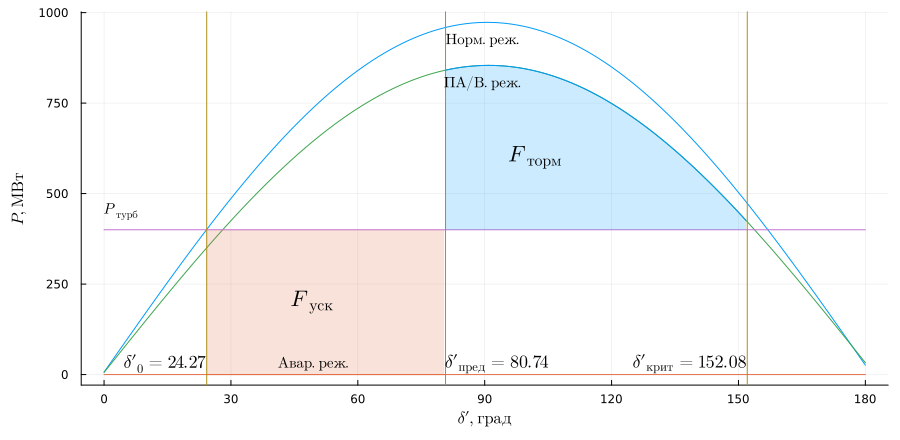
d_pr = acos((P0 * 1e-6 * (pi - d0_pav - d0p) + Pmax_pav * cos(pi - d0_pav) - Pmax_av * cos(d0p)) / (Pmax_pav - Pmax_av));
Visualization of the area method:
# functions of angular characteristics
delta = 0:0.1:180
Pmax = x -> (Eqq ^ 2 / abs(Z11) * sin(alpha11) .+ (Eqq * Us / abs(Z12)) * sin.(x .- alpha12)) / 1e6
Pmax_av = x -> fill(0, size(x))
Pmax_pav = x -> (Eqq_pav ^ 2 / abs(Z11_pav) * sin(alpha11_pav) .+ Eqq_pav * Us / abs(Z12_pav) * sin.(x .- alpha12_pav)) / 1e6
Pt = x -> fill(P0 * 1e-6, size(x))
# visualization of the area method
plot(delta, [Pmax(delta .* pi ./ 180) Pmax_av(delta .* pi ./ 180) Pmax_pav(delta .* pi ./ 180) Pt(delta)],
label = [L"Norm.dir." L"Avar.dir." L"N/A.dir." L"Powerful.turbines"], ylabel = L"P, MW", xlabel = L"\delta\prime, hail", legend=false,
xaxis = (0:30:180), size = (900,440), left_margin=5Plots.mm, bottom_margin=5Plots.mm)
plot!((d0p:0.01:d_pr) .* 180 / pi, Pmax_av((d0p:0.01:d_pr)), fillrange = Pt((d0p:0.01:d_pr)), fillalpha = 0.2, c = 2, label = "Ftorm")
plot!((d_pr:0.01:dkr) .* 180 / pi, Pmax_pav((d_pr:0.01:dkr)), fillrange = Pt((d_pr:0.01:dkr)), fillalpha = 0.2, c = 1, label = "Ftorm")
vline!([d0p,d_pr,dkr] .* 180 / pi, c = 5)
annotate!([(90, Pmax(pi / 2) - 50, (L"Norm.dir.", 10, :black)),
        (50, Pmax_av(pi / 2) .+ 30, (L"Avar.dir.", 10, :black)),
        (90, Pmax_pav(pi / 2) - 50, (L"PA/V.dir.", 10, :black)),
        (d0p * 180 / pi + 20, P0 * 1e-6 - 200, (L"F_{usk}", 15, :black, :left)),
        (d_pr * 180 / pi + 15, P0 * 1e-6 + 200, (L"F_{torm}", 15, :black, :left)),
        (0, P0 * 1e-6 + 50, (L"P_{turb}", 10, :black, :left)),
        (d0p * 180 / pi, 30, (L"\delta\prime_0  = %$(round(d0p * 180 / pi, digits=2))", 12, :black, :right)),
        (d_pr * 180 / pi, 30, (L"\delta\prime_{pre} = %$(round(d_pr * 180 / pi, digits=2))", 12, :black, :left)),
        (dkr * 180 / pi, 30, (L"\delta\prime_{crete} = %$(round(dkr * 180 / pi, digits=2))", 12, :black, :right))])
The maximum shutdown time of the short circuit:
Tj = 7.05
tpr = sqrt((d_pr - d0p) * 2 * Tj / (0.8 * 2 * pi * 50))
print("t_pred = $(round(tpr, digits = 3))")
Simulation
Loading the model:
model_name = "synchronous_generator_round_rotor";
model_name in [m.name for m in engee.get_all_models()] ? engee.open(model_name) : engee.load( "$(@__DIR__)/$(model_name).engee");
Setting the model using command control for the time of line disconnection and short circuit equal to 0.24 seconds, at which dynamic stability will be maintained:
step = "Short circuit shutdown";
# disconnecting the overhead line circuit
engee.set_param!(model_name * "/" * step, "Time" => 5.24);
Launching the uploaded model:
results = engee.run(model_name);
To import the simulation results, logging of the necessary signals was enabled in advance and their names were set. Converting the simulation results from the results variable:
# simulation time vector
sim_time = results["w"].time;
# vector of rotation speed of the rotor
w1 = results["w"].value;
# generator current vector
P1 = results["P"].value;
Simulation with an increase in the short circuit duration to 0.2402 s:
# disconnecting the overhead line circuit
engee.set_param!(model_name*"/"*step, "Time" => 5.2402);
results = engee.run(model_name);
# vector of rotation speed of the rotor
w2 = results["w"].value;
# generator current vector
P2 = results["P"].value;
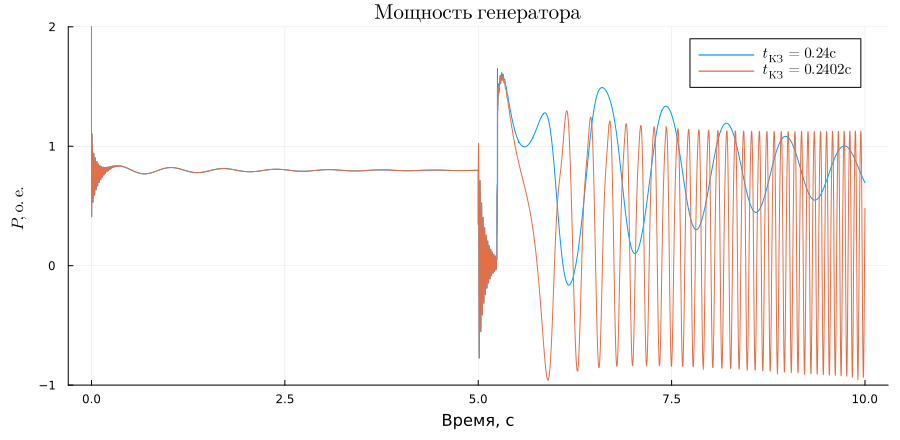
Graphs of the generator's active power:
plot(sim_time, P1, title = L"Generator power", ylabel = L"P, O.E.", xlabel="Time, c",  label = L"t_{short circuit} = 0.24 s", legendfontsize = 10)
plot!(sim_time, P2,  label = L"t_{short circuit} = 0.2402 s", ylims = (-1, 2),size = (900,440), left_margin=5Plots.mm, bottom_margin=5Plots.mm)
Rotor speed charts:
plot(sim_time, w1, title = L"Speed of the rotor", ylabel = L"\omega, O.E.", xlabel=L"Time, c", label = L"t_{short circuit} = 0.24 s", legendfontsize = 10)
plot!(sim_time, w2, label = L"t_{short circuit} = 0.2402 s", ylims = (0.95, 1.1),size = (900,440), left_margin=5Plots.mm, bottom_margin=5Plots.mm)
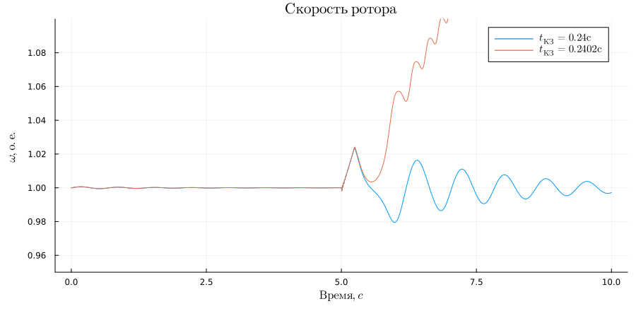
In the second experiment, the dynamic stability of the generator was disrupted, so the maximum short-circuit shutdown time in the model was empirically found. The result is consistent with the theoretical calculation with a small margin of error.
println("Limit shutdown time analytically = "*string(round(tpr, digits=3)) * "with")
println("The maximum shutdown time is practically = "*string(0.24) * "with")
Addition
Try to change the following model parameters yourself and explore how this affects dynamic stability:
- increase overhead line length by 200 km;
- Type of fault in the Fault (Three-Phase) block;
- Reduce the active power of the generator in the initial mode by 200 MW.
Conclusions
In this example, tools were used for command management of the Engee model and uploading simulation results, and work with the Plots module is shown. The operation of an implicit-pole generator through a transformer and a two-circuit overhead line on a BWM without regulators of excitation and rotation speed was considered. The analytical calculation of dynamic stability was carried out and the results were compared with the modeling data.
Links
- Venikov V. A. Transient electromechanical processes in electrical systems: Textbook for electric power industry. spec. universities. — 4th ed., revised and dop. — M.: Higher School, 1985
- Transient processes of electrical systems in examples and illustrations: A textbook for universities (V. V. Yezhkov, N. I. Zelenokhat, I. V. Litkens, and others; edited by V. A. Stroev). Moscow: Znak, 1996. 224s., ill.
- Dolgov A.P. Stability of electrical systems : a textbook / Dolgov A.P.. Novosibirsk : Novosibirsk State Technical University, 2010. 177 p. ISBN 978-5-7782-1320-3.