Damage in the network with an isolated neutral conductor
Description of the model
This example examines the damage in a network with an isolated neutral. The model is a 110/10 kV step-down substation and a 10 kV distribution network with three feeders. At a time of 0.2 s, a single-phase earth fault occurs in phase A at the end of the cable line (CL) 4 of the third feeder, then at a time of 0.5 s at the end of CL 2 of the first feeder, an earth fault occurs in phase B, which creates a circuit for short-circuit currents to flow between phases A and B. At a time of 1 s with a difference of 100 ms, the switches on the first and third feeders are switched off, simulating the operation of relay protection and eliminating a double earth fault. The example shows the process of launching a model from the script development environment using command control and visualization of simulation results. The model measures currents and voltages at the beginning of each of the feeders. The model's appearance:
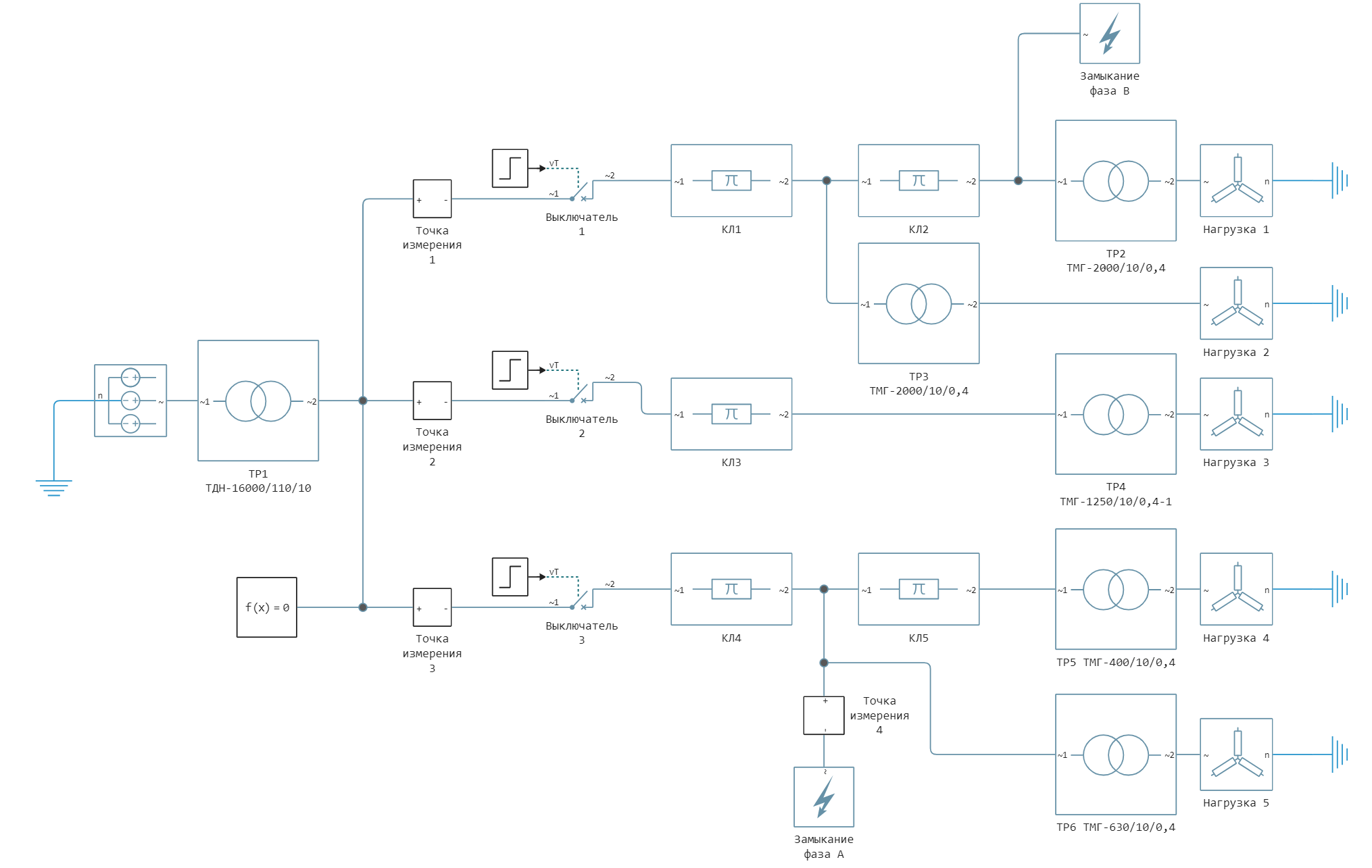
The power supply is modeled by a block Voltage Source (Three-Phase). Cable lines are modeled by a block Three-Phase PI Section Line. Transformers are modeled by a block Three-Phase Transformer (Two Windings). Closures are modeled by the block Fault (Three-Phase) in the settings of this block, using the Failure mode drop-down menu, you can select the type of short circuit. Disconnection of the circuit occurs using the block Circuit Breaker (Three-Phase), which simulates disconnection from relay protection. The load is modeled by the block Wye-Connected Load.
System parameters [1,2]:
| Element | Parameter |
|---|---|
| System | Balancing node |
| TR 1 | TDN-16000/110/10 |
| TR 2 | TMG-2000/10/0.4 |
| TR 3 | TMG-2000/10/0.4 |
| TR 4 | TMG-1250/10/0.4 |
| TR 5 | TMG-400/10/0.4 |
| TR 6 | TMG-630/10/0.4 |
| CLASS 1 | 3xAPvV 1x240; |
| CLASS 2 | 3xAPvV 1x120; |
| CLASS 3 | 3xAPvV 1x95; |
| CLASS 4 | 3xAPvV 1x70; |
| CLASS 5 | 3xAPvV 1x70; |
| Load 1 | |
| Load 2 | |
| Load 3 | |
| Load 4 | |
| Load 5 |
Launching the model
Importing the necessary modules for working with graphs and LaTex strings:
using Plots
using LaTeXStrings
gr();
Loading the model:
model_name = "isolated_neutral_network_fault"
model_name in [m.name for m in engee.get_all_models()] ? engee.open(model_name) : engee.load( "$(@__DIR__)/$(model_name).engee");
Launching the uploaded model:
results = engee.run(model_name);
Simulation results
To import the simulation results, the recording of the necessary signals was enabled in advance and their names were set. We convert the instantaneous values of currents and voltages of the results variable into separate vectors:
# simulation time vector
sim_time = results["i_a_1"].time;
# vectors of currents and voltages at the measuring point 1
i_1 = hcat(results["i_a_1"].value,results["i_b_1"].value,results["i_c_1"].value,results["3I0_1"].value);
v_1 = hcat(results["v_a_1"].value,results["v_b_1"].value,results["v_c_1"].value);
# vectors of currents and voltages at the measuring point 3
i_3 = hcat(results["i_a_3"].value,results["i_b_3"].value,results["i_c_3"].value,results["3I0_3"].value);
v_3 = hcat(results["v_a_3"].value,results["v_b_3"].value,results["v_c_3"].value,results["3V0_3"].value);
Graphs of feeder 3 currents and bus voltage NN PS:
p1 = plot(sim_time, v_3[:,1:3]./1e3, label = [L"U_a" L"U_b" L"U_c"],
title = "Voltage", linecolor = [:orange :green :red], ylabel = "U, kV", xlabel="Time, c");
p2 = plot(sim_time, i_3[:,1:3], label = [L"I_a" L"I_b" L"I_c"],
title = "Currents", linecolor = [:orange :green :red], ylabel = "I, And", xlabel="Time, c");
plot(p1, p2, layout=(2,1),legend = true, size = (750,440))
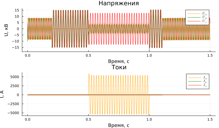
When phase A is closed to earth, the voltage in this phase relative to earth becomes zero, as a result, the voltage of the intact phases becomes linear. This is one of the disadvantages of networks with an isolated neutral. At a time of 0.5 s, when an earth fault occurs in phase B, a single-phase short circuit transitions to a double one at the end of the first feeder circuit. The voltage of the damaged phases is significantly reduced due to a multiple increase in short-circuit currents.
NP voltage graph on NN PS busbars:
plot(sim_time, v_3[:,4]./1e3, label = L"3U_0", title = L"3U_0", linecolor = :orange, ylabel = "U, kV", xlabel="Time, c")
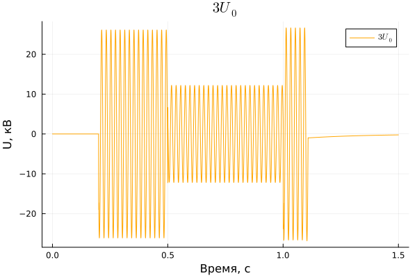
The NP voltage waveform corresponds to the OZZ. The voltage of the NP on the PS busbars is used to determine the presence of an OPZ in the network.
Graph of the current of the zero sequence (NP) of the third feeder in the time interval from 0 to 0.4 s:
plot(sim_time[1:Int(indexin(0.4, sim_time)[1])],
i_3[1:Int(indexin(0.4, sim_time)[1]),4], title = L"3I_0",
linecolor = :orange, ylabel = "I, And", xlabel="Time, c", legend = false)
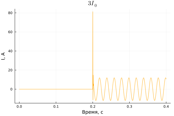
The NP current appears due to capacitive currents between the intact phases and the ground. If its value is small, as in this example, then it is not necessary to disconnect this circuit instantly. Due to the small value of the OZZ current, the line voltages remain unchanged in magnitude and shifted in phase by an angle of 120 °. These circumstances make it possible to maintain the power supply to consumers until the fault location is detected. Due to the connection of the windings of all transformers in a triangle on the side of the 10 kV network, the windings are isolated from the ground and no NP current passes through the transformers.
Graph of NP currents of feeders 1 and 3 in the time interval from 0.4 to 1.5 s:
p1 = plot(sim_time[Int(indexin(0.4, sim_time)[1]):end], i_1[Int(indexin(0.4, sim_time)[1]):end,4],
title = L"3I_0(feeder\,1)", ylabel = "I, And", xlabel="Time, c")
p2 = plot(sim_time[Int(indexin(0.4, sim_time)[1]):end], i_3[Int(indexin(0.4, sim_time)[1]):end,4],
title = L"3I_0(feeder\,3)", ylabel = "I, And", xlabel="Time, c")
plot(p1, p2, layout = (2,1), legend=false, size = (750,440))
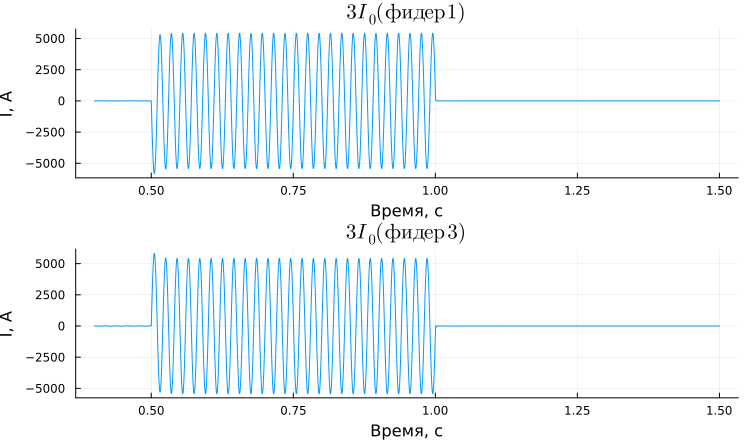
When a second earth fault occurs in phase B, a circuit appears for fault current to flow through the ground between phases A and B. The large value of the fault current is due to the low resistance of the current circuit consisting of resistances KL1, KL2, KL4 and TR1.
Addition
Try to change the following model parameters yourself and investigate how this affects the currents and voltages during OPW:
- Double the length of the cable lines;
- Move the short circuit block in phase B to the TP1 bus.
Conclusion
In this example, the process of switching a single-phase earth fault to a double one was shown. The Engee model command management tools are used to download and run the model from the script development environment. The measured currents and voltages were imported into the Workspace from the result variable and displayed on time graphs.
Links
- Handbook on the design of electrical networks /
edited by D. L. Faybisovich. – 4th ed., revised and add. – M. : ENAS, 2012. – 376 p. : ill. - The designer's desktop book. Cross-linked polyethylene insulated cables with a voltage of 6-35 kV. Kamsky Cable LLC. URL: https://www.kamkabel.ru/netcat_files/userfiles/6-35-www.pdf?ysclid=m2j0odmzen889432059 (accessed on 10/21/2024).