Short-circuit current transfer through transformer
Description of the model
In this example, we consider a power system with an overhead line with one-way power supply and a two-winding transformer, behind which various types of short circuits occur. The process of launching, editing the model from the script development environment using command control, and visualizing the simulation results are shown. The model measures the currents on the sides of the high voltage (OH) and low voltage (OH) transformer, then shows their time graphs and vector diagrams. The model's appearance:
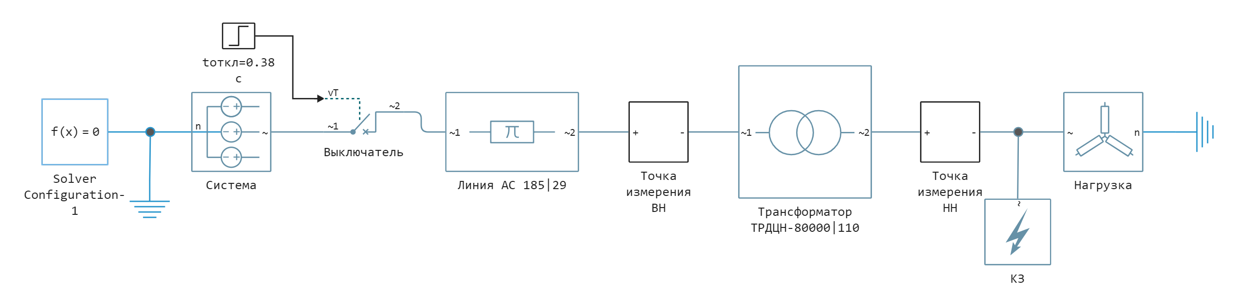
The power supply is modeled by a block Voltage Source (Three-Phase). The overhead line is modeled by a block Three-Phase PI Section Line. A short circuit is modeled by a block Fault (Three-Phase) in the settings of this block, using the Filure mode drop-down menu, you can select the type of short circuit. The short circuit is disabled using the block Circuit Breaker (Three-Phase), which simulates the operation of relay protection. The duration of the short-circuit shutdown is selected based on the operating time of the dead-end line protections with one-way power supply and the switch-off time, and is set to 0.18 s at the upper limit of the short-circuit shutdown duration for 110 kV in accordance with the Methodological Guidelines on the Stability of Power Systems from 2003 [1]. The load is modeled by the block Wye-Connected Load.
System parameters [2]:
| Element | Parameter |
|---|---|
| System | Balancing node |
| Line | AC 185/29 |
| Transformer | TRDCN-80000/110 |
| Load | |
Launching the model
We will import the necessary modules for working with graphs, tables, and a floating-window Fourier transform function.:
using Plots
using DataFrames
include("$(@__DIR__)/fourie_func.jl")
gr();
Loading the model:
model_name = "transformer_fault"
model_name in [m.name for m in engee.get_all_models()] ? engee.open(model_name) : engee.load( "$(@__DIR__)/$(model_name).engee");
Setting up the model for the first experience with 3-F short circuit and winding connection scheme :
transf_name = "Transformer TRDCN-80000/110";
fault_name = "KZ";
line_name = "Line AC 185/29"
engee.set_param!(model_name*"/"*transf_name,
"winding1_connection" => "Wye with grounded neutral",
"winding2_connection" => "Delta 11 o'clock");
engee.set_param!(model_name*"/"*fault_name, "type" => "Three-phase (a-b-c)");
engee.set_param!(model_name*"/"*line_name, "line_length" => 20);
Launching the uploaded model:
results = engee.run(model_name);
Simulation results
To import the simulation results, logging of the necessary signals was enabled in advance and their names were set. Converting the instantaneous values of the currents of the results variable into separate vectors:
# simulation time vector
sim_time = results["i_a_1"].time;
# the vector of currents on the VN side
i_1 = hcat(results["i_a_1"].value,results["i_b_1"].value,results["i_c_1"].value);
# the vector of currents on the VN side
i_2 = hcat(results["i_a_2"].value,results["i_b_2"].value,results["i_c_2"].value);
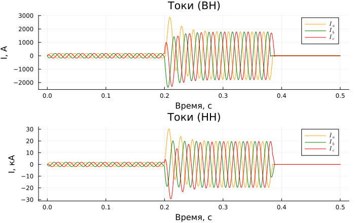
Graphs of currents from the side of VN and NN:
p1 = plot(sim_time, i_1, label = [L"I_a" L"I_b" L"I_c"],
title = "Currents (VN)", ylabel = "I, And", xlabel="Time, c");
p2 = plot(sim_time, i_2./1e3, label = [L"I_a" L"I_b" L"I_c"],
title = "Currents (NN)", ylabel = "I, kA", xlabel="Time, c")
plot(p1, p2, layout=(2,1), legend = true, linecolor = [:orange :green :red], size = (700,440))
Let's perform vectorization of currents using a Fourier transform with a floating window to isolate the amplitudes and phases of currents.
At the same time, we will not use the built-in functions and will use the function [3]:
# Variables for storing vectors
i_1_Xmag, i_2_Xmag,
i_1_Xphase, i_2_Xphase = [zeros(length(sim_time),3) for _ = 1:4];

for (Xmag, Xphase, signal) in zip(
    (i_1_Xmag, i_2_Xmag),
    (i_1_Xphase, i_2_Xphase),
    (i_1, i_2))
    Xmag, Xphase = moving_fourie(Xmag, Xphase, sim_time, signal);
end
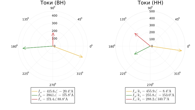
For greater clarity, the currents from the HH side are reduced to the HH side by dividing by the transformation coefficient. Vector diagrams of currents on the sides of VN and NN during short circuit:
# KZ index search
fault_ind = indexin(0.3, sim_time);
# transformation coefficient
kt = 115/10.5;
# vectors of currents in complex numbers
i_a_HV_mag, i_a_HV_ang = round(i_1_Xmag[fault_ind,1][1], digits=1), round(i_1_Xphase[fault_ind,1][1], digits=1)
i_b_HV_mag, i_b_HV_ang = round(i_1_Xmag[fault_ind,2][1], digits=1), round(i_1_Xphase[fault_ind,2][1], digits=1)
i_c_HV_mag, i_c_HV_ang = round(i_1_Xmag[fault_ind,3][1], digits=1), round(i_1_Xphase[fault_ind,3][1], digits=1)
i_a_LV_mag, i_a_LV_ang = round(i_2_Xmag[fault_ind,1][1]/kt, digits=1), round(i_2_Xphase[fault_ind,1][1], digits=1)
i_b_LV_mag, i_b_LV_ang = round(i_2_Xmag[fault_ind,2][1]/kt, digits=1), round(i_2_Xphase[fault_ind,2][1], digits=1)
i_c_LV_mag, i_c_LV_ang = round(i_2_Xmag[fault_ind,3][1]/kt, digits=1), round(i_2_Xphase[fault_ind,3][1], digits=1)

p1 = plot([0;i_a_HV_ang*pi/180], [0;i_a_HV_mag], arrow=true, proj = :polar, linecolor = :orange,
label = L"I_a = %$i_a_HV_mag \angle\, %$i_a_HV_ang\degree And", title = "Currents (VN)")

plot!([0;i_b_HV_ang*pi/180], [0;i_b_HV_mag], arrow=true, proj = :polar, linecolor = :green,
label = L"I_b = %$i_b_HV_mag \angle\, %$i_b_HV_ang \degree And")

plot!([0;i_c_HV_ang*pi/180], [0;i_c_HV_mag], arrow=true, proj = :polar, linecolor = :red,
label = L"I_c = %$i_c_HV_mag \angle\, %$i_c_HV_ang \degree And")

p2 = plot([0;i_a_LV_ang*pi/180], [0;i_a_LV_mag], arrow=true, proj = :polar, linecolor = :orange,
label = L"I_a/k_t = %$i_a_LV_mag \angle\, %$i_a_LV_ang\degree And", title = "Currents (NN)")

plot!([0;i_b_LV_ang*pi/180], [0;i_b_LV_mag], arrow=true, proj = :polar, linecolor = :green,
label = L"I_b/k_t = %$i_b_LV_mag \angle\, %$i_b_LV_ang\degree And")

plot!([0;i_c_LV_ang*pi/180], [0;i_c_LV_mag], arrow=true, proj = :polar, linecolor = :red,
label = L"I_c/k_t = %$i_c_LV_mag \angle\, %$i_c_LV_ang\degree And")

plot(p1, p2, layout=(1,2), legend = :outerbottom, legendfontsize=10, size = (800,450))
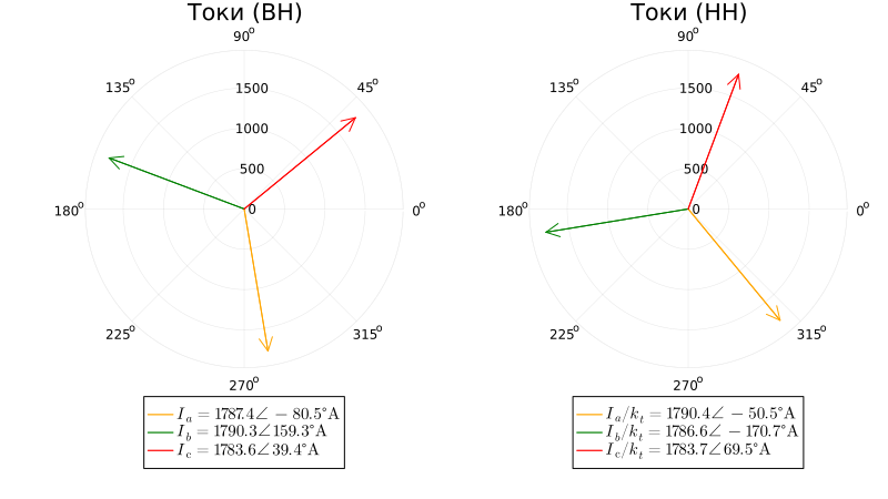
Pay attention to the symmetry of the short-circuit currents and the phase shift of the currents on the HH side relative to the currents on the HH side by due to the connection scheme of the windings . In this case, the linear currents from the sides of the VN and NN during the transition through the transformer are equal, taking into account the transformation coefficient, and the phase currents from the NN side are less than linear.
Experience with 2-F short circuit and winding connection scheme
Setting up a model for an experiment with 2-F short circuits and a winding connection scheme :
engee.set_param!(model_name*"/"*transf_name,
"winding1_connection" => "Wye with grounded neutral",
"winding2_connection" => "Delta 11 o'clock");
engee.set_param!(model_name*"/"*fault_name, "type" => "Two-phase (b-c)");
Model launch, processing, and vectorization of measured currents:
results = engee.run(model_name);
# current vector of the ammeter 1
i_1 = hcat(results["i_a_1"].value,results["i_b_1"].value,results["i_c_1"].value);
# current vector of the ammeter 2
i_2 = hcat(results["i_a_2"].value,results["i_b_2"].value,results["i_c_2"].value);

for (Xmag, Xphase, signal) in zip(
    (i_1_Xmag, i_2_Xmag),
    (i_1_Xphase, i_2_Xphase),
    (i_1, i_2))
    Xmag, Xphase = moving_fourie(Xmag, Xphase, sim_time, signal);
end
Vector diagram of currents on the sides of VN and NN during short circuit:
# vectors of currents in complex numbers
i_a_HV_mag, i_a_HV_ang = round(i_1_Xmag[fault_ind,1][1], digits=1), round(i_1_Xphase[fault_ind,1][1], digits=1)
i_b_HV_mag, i_b_HV_ang = round(i_1_Xmag[fault_ind,2][1], digits=1), round(i_1_Xphase[fault_ind,2][1], digits=1)
i_c_HV_mag, i_c_HV_ang = round(i_1_Xmag[fault_ind,3][1], digits=1), round(i_1_Xphase[fault_ind,3][1], digits=1)
i_a_LV_mag, i_a_LV_ang = round(i_2_Xmag[fault_ind,1][1]/kt, digits=1), round(i_2_Xphase[fault_ind,1][1], digits=1)
i_b_LV_mag, i_b_LV_ang = round(i_2_Xmag[fault_ind,2][1]/kt, digits=1), round(i_2_Xphase[fault_ind,2][1], digits=1)
i_c_LV_mag, i_c_LV_ang = round(i_2_Xmag[fault_ind,3][1]/kt, digits=1), round(i_2_Xphase[fault_ind,3][1], digits=1)

p1 = plot([0;i_a_HV_ang*pi/180], [0;i_a_HV_mag], arrow=true, proj = :polar, linecolor = :orange,
label = L"I_a = %$i_a_HV_mag \angle\, %$i_a_HV_ang\degree And", title = "Currents (VN)")

plot!([0;i_b_HV_ang*pi/180], [0;i_b_HV_mag], arrow=true, proj = :polar, linecolor = :green,
label = L"I_b = %$i_b_HV_mag \angle\, %$i_b_HV_ang \degree And")

plot!([0;i_c_HV_ang*pi/180], [0;i_c_HV_mag], arrow=true, proj = :polar, linecolor = :red,
label = L"I_c = %$i_c_HV_mag \angle\, %$i_c_HV_ang \degree And")

p2 = plot([0;i_a_LV_ang*pi/180], [0;i_a_LV_mag], arrow=true, proj = :polar, linecolor = :orange,
label = L"I_a/k_t = %$i_a_LV_mag \angle\, %$i_a_LV_ang\degree And", title = "Currents (NN)")

plot!([0;i_b_LV_ang*pi/180], [0;i_b_LV_mag], arrow=true, proj = :polar, linecolor = :green,
label = L"I_b/k_t = %$i_b_LV_mag \angle\, %$i_b_LV_ang\degree And")

plot!([0;i_c_LV_ang*pi/180], [0;i_c_LV_mag], arrow=true, proj = :polar, linecolor = :red,
label = L"I_c/k_t = %$i_c_LV_mag \angle\, %$i_c_LV_ang\degree And")

plot(p1, p2, layout=(1,2), legend = :outerbottom, legendfontsize=10, size = (800,450))
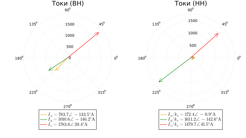
At 2-f short circuit, currents of the reverse sequence appear, equal to the currents of the forward sequence. The position of the vector diagram of the reverse sequence currents at the short–circuit location is determined taking into account a special condition - the short-circuit current in the intact phase is zero . Therefore, the current vectors of the forward and reverse sequences for this phase should be directed in opposite directions. As a result of the vector addition of the symmetrical components, the currents of phases A and B on the side of the high voltage are practically two times less than the current in phase C.
Experience with 1-f short circuit and winding connection scheme
Setting up a model for an experiment with 1-f short circuit and a winding connection scheme :
engee.set_param!(model_name*"/"*transf_name,
"winding1_connection" => "Wye with grounded neutral",
"winding2_connection" => "Delta 11 o'clock");
engee.set_param!(model_name*"/"*fault_name, "type" => "Single-phase to ground (a-g)");
Model launch, processing, and vectorization of measured currents:
results = engee.run(model_name);
# current vector of the ammeter 1
i_1 = hcat(results["i_a_1"].value,results["i_b_1"].value,results["i_c_1"].value);
# current vector of the ammeter 2
i_2 = hcat(results["i_a_2"].value,results["i_b_2"].value,results["i_c_2"].value);

for (Xmag, Xphase, signal) in zip(
    (i_1_Xmag, i_2_Xmag),
    (i_1_Xphase, i_2_Xphase),
    (i_1, i_2))
    Xmag, Xphase = moving_fourie(Xmag, Xphase, sim_time, signal);
end
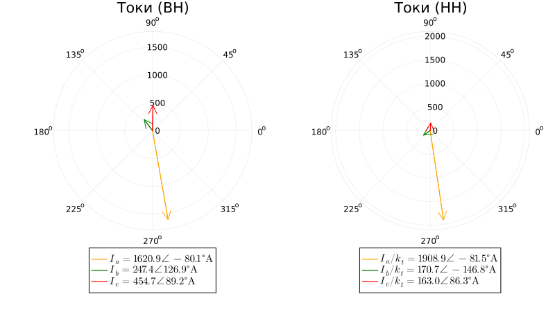
Vector diagram of currents on the sides of VN and NN during short circuit:
# vectors of currents in complex numbers
i_a_HV_mag, i_a_HV_ang = round(i_1_Xmag[fault_ind,1][1], digits=1), round(i_1_Xphase[fault_ind,1][1], digits=1)
i_b_HV_mag, i_b_HV_ang = round(i_1_Xmag[fault_ind,2][1], digits=1), round(i_1_Xphase[fault_ind,2][1], digits=1)
i_c_HV_mag, i_c_HV_ang = round(i_1_Xmag[fault_ind,3][1], digits=1), round(i_1_Xphase[fault_ind,3][1], digits=1)
i_a_LV_mag, i_a_LV_ang = round(i_2_Xmag[fault_ind,1][1]/kt, digits=1), round(i_2_Xphase[fault_ind,1][1], digits=1)
i_b_LV_mag, i_b_LV_ang = round(i_2_Xmag[fault_ind,2][1]/kt, digits=1), round(i_2_Xphase[fault_ind,2][1], digits=1)
i_c_LV_mag, i_c_LV_ang = round(i_2_Xmag[fault_ind,3][1]/kt, digits=1), round(i_2_Xphase[fault_ind,3][1], digits=1)

p1 = plot([0;i_a_HV_ang*pi/180], [0;i_a_HV_mag], arrow=true, proj = :polar, linecolor = :orange,
label = L"I_a = %$i_a_HV_mag \angle\, %$i_a_HV_ang\degree And", title = "Currents (VN)")

plot!([0;i_b_HV_ang*pi/180], [0;i_b_HV_mag], arrow=true, proj = :polar, linecolor = :green,
label = L"I_b = %$i_b_HV_mag \angle\, %$i_b_HV_ang \degree And")

plot!([0;i_c_HV_ang*pi/180], [0;i_c_HV_mag], arrow=true, proj = :polar, linecolor = :red,
label = L"I_c = %$i_c_HV_mag \angle\, %$i_c_HV_ang \degree And")

p2 = plot([0;i_a_LV_ang*pi/180], [0;i_a_LV_mag], arrow=true, proj = :polar, linecolor = :orange,
label = L"I_a/k_t = %$i_a_LV_mag \angle\, %$i_a_LV_ang\degree And", title = "Currents (NN)")

plot!([0;i_b_LV_ang*pi/180], [0;i_b_LV_mag], arrow=true, proj = :polar, linecolor = :green,
label = L"I_b/k_t = %$i_b_LV_mag \angle\, %$i_b_LV_ang\degree And")

plot!([0;i_c_LV_ang*pi/180], [0;i_c_LV_mag], arrow=true, proj = :polar, linecolor = :red,
label = L"I_c/k_t = %$i_c_LV_mag \angle\, %$i_c_LV_ang\degree And")

plot(p1, p2, layout=(1,2), legend = :outerbottom, legendfontsize=10, size = (800,450))
In this example, there is a load with a neutral point ground, which forms a circuit for the flow of currents during a single-phase earth fault, however, the zero-sequence current closes in the NN winding and does not pass to the VN side.
Addition
Try to change the characteristics of the system and explore how this will affect the parameters of the power system mode:
# @markdown Length of overhead line, in km:
L1 = 20 # @param {type:"slider", min:1, max:100, step:1}
engee.set_param!(model_name*"/"*line_name, "line_length" => float(L1));
# @markdown Connection diagram of the windings on the VN side:
winding_con_HV = "Wye with grounded neutral" # @param ["Wye with floating neutral", "Wye with grounded neutral", "Delta 1 o'clock", "Delta 11 o'clock"]
# @markdown Connection diagram of the windings on the NN side:
winding_con_LV = "Wye with grounded neutral" # @param ["Wye with floating neutral", "Wye with grounded neutral", "Delta 1 o'clock", "Delta 11 o'clock"]
engee.set_param!(model_name*"/"*transf_name,
"winding1_connection" => winding_con_HV,
"winding2_connection" => winding_con_LV);
# @markdown Short-circuit view
kind_of_fault = "Single-phase to ground (a-g)" # @param ["Single-phase to ground (a-g)", "Single-phase to ground (b-g)", "Single-phase to ground (c-g)", "Two-phase (a-b)", "Two-phase (b-c)", "Two-phase (c-a)", "Three-phase (a-b-c)", "Three-phase ground (a-b-c-g)"]
engee.set_param!(model_name*"/"*fault_name, "type" => kind_of_fault);
Model launch, processing, and vectorization of measured currents:
results = engee.run(model_name);
# the vector of currents on the VN side
i_1 = hcat(results["i_a_1"].value,results["i_b_1"].value,results["i_c_1"].value);
# the vector of currents on the NN side
i_2 = hcat(results["i_a_2"].value,results["i_b_2"].value,results["i_c_2"].value);

for (Xmag, Xphase, signal) in zip(
    (i_1_Xmag, i_2_Xmag),
    (i_1_Xphase, i_2_Xphase),
    (i_1, i_2))
    Xmag, Xphase = moving_fourie(Xmag, Xphase, sim_time, signal);
end
Vector diagram of currents on the sides of VN and NN during short circuit:
# vectors of currents in complex numbers
i_a_HV_mag, i_a_HV_ang = round(i_1_Xmag[fault_ind,1][1], digits=1), round(i_1_Xphase[fault_ind,1][1], digits=1)
i_b_HV_mag, i_b_HV_ang = round(i_1_Xmag[fault_ind,2][1], digits=1), round(i_1_Xphase[fault_ind,2][1], digits=1)
i_c_HV_mag, i_c_HV_ang = round(i_1_Xmag[fault_ind,3][1], digits=1), round(i_1_Xphase[fault_ind,3][1], digits=1)
i_a_LV_mag, i_a_LV_ang = round(i_2_Xmag[fault_ind,1][1]/kt, digits=1), round(i_2_Xphase[fault_ind,1][1], digits=1)
i_b_LV_mag, i_b_LV_ang = round(i_2_Xmag[fault_ind,2][1]/kt, digits=1), round(i_2_Xphase[fault_ind,2][1], digits=1)
i_c_LV_mag, i_c_LV_ang = round(i_2_Xmag[fault_ind,3][1]/kt, digits=1), round(i_2_Xphase[fault_ind,3][1], digits=1)

p1 = plot([0;i_a_HV_ang*pi/180], [0;i_a_HV_mag], arrow=true, proj = :polar, linecolor = :orange,
label = L"I_a = %$i_a_HV_mag \angle\, %$i_a_HV_ang\degree And", title = "Currents (VN)")

plot!([0;i_b_HV_ang*pi/180], [0;i_b_HV_mag], arrow=true, proj = :polar, linecolor = :green,
label = L"I_b = %$i_b_HV_mag \angle\, %$i_b_HV_ang \degree And")

plot!([0;i_c_HV_ang*pi/180], [0;i_c_HV_mag], arrow=true, proj = :polar, linecolor = :red,
label = L"I_c = %$i_c_HV_mag \angle\, %$i_c_HV_ang \degree And")

p2 = plot([0;i_a_LV_ang*pi/180], [0;i_a_LV_mag], arrow=true, proj = :polar, linecolor = :orange,
label = L"I_a/k_t = %$i_a_LV_mag \angle\, %$i_a_LV_ang\degree And", title = "Currents (NN)")

plot!([0;i_b_LV_ang*pi/180], [0;i_b_LV_mag], arrow=true, proj = :polar, linecolor = :green,
label = L"I_b/k_t = %$i_b_LV_mag \angle\, %$i_b_LV_ang\degree And")

plot!([0;i_c_LV_ang*pi/180], [0;i_c_LV_mag], arrow=true, proj = :polar, linecolor = :red,
label = L"I_c/k_t = %$i_c_LV_mag \angle\, %$i_c_LV_ang\degree And")

plot(p1, p2, layout=(1,2), legend = :outerbottom, legendfontsize=10, size = (800,450))
Conclusion
In this example, the features of the short-circuit current transition through a transformer were shown. The Engee model command management tools are used to load and run the model and configure blocks from the script development environment. The measured currents were imported into the Workspace from the result variable and displayed on time graphs. They were then vectorized using a Fourier transform with a floating window and shown on vector diagrams. Visualization was performed using the Plots module. The Addition section uses masked code cells to improve the interactivity of the example.
Links
- Methodological guidelines on the stability of energy systems.
Approved by the Order of the Ministry of Energy of Russia dated June 30, 2003 N 277. - Handbook on the design of electrical networks /
edited by D. L. Faybisovich. – 4th ed., revised and add. – M. : ENAS, 2012. – 376 p. : ill. - Microprocessor relays: a textbook / A. A. Nikitin; Ministry of Education and Science of the Russian Federation, Federal Agency for Education, Federal State Educational Institution of Higher Professional Education. education "Chuvash State University named after I. N. Ulyanov". Cheboksary : Publishing House of the Chuvash University, 2006. 447 p.; ISBN 5-7677-1051-1