A power system model with a simplified synchronous generator
In this example, we will consider a synchronous generator (power_ssm.engee model) P=20 kW U= 24 kV, on the buses of which a base load (P= 10 kW and Q=100 Var) and a switching load (P=10 kW and Q=100 Var) are connected at time 0.1 (model power_ssm.engee).
Implementation of the model launch using software control:
Pkg.add(["Statistics"])
using Plots
using DataFrames
using Statistics
gr();
Loading the model:
model_name = "power_ssm"
model_name in [m.name for m in engee.get_all_models()] ? engee.open(model_name) : engee.load( "$(@__DIR__)/$(model_name).engee");
Launching the uploaded model:
results = engee.run(model_name)
Reading data on instantaneous current and voltage values:
t = results["i_a"].time;
i_a = results["i_a"].value;
i_b = results["i_b"].value;
i_c = results["i_c"].value;
v_a = results["v_a"].value;
v_b = results["v_b"].value;
v_c = results["v_c"].value;
Downloading and visualizing the data obtained during the simulation
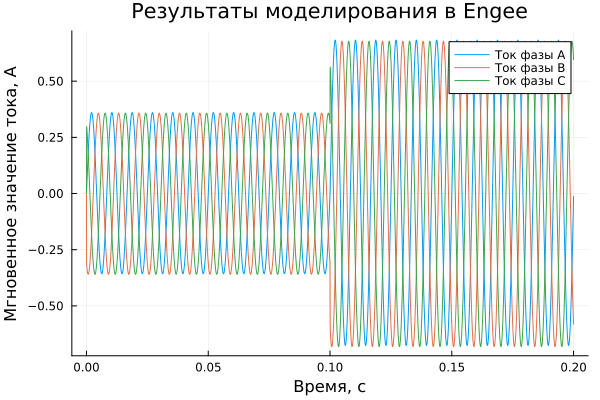
Output of a graph of the dependence of instantaneous current values on time:
plot(t, [i_a i_b i_c], label=["Phase A current" "Phase V current" "Phase C current"])
plot!(title = "Simulation results in Engee", ylabel = "The instantaneous value of the current, And", xlabel="Time, c")
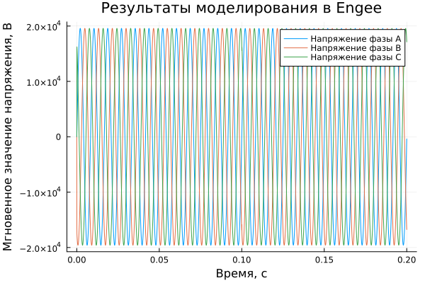
Output of a graph of the dependence of instantaneous voltage values on time:
plot(t, [v_a v_b v_c], label=["Phase A voltage" "Phase voltage V" "Phase C voltage"])
plot!(title = "Simulation results in Engee", ylabel = "Instantaneous voltage value, In", xlabel="Time, c")
Conclusions:
In this example, tools for command management of the Engee model were used. The model demonstrates the operation of a synchronous generator on a load that varies by leaps and bounds. The simulation results were imported into an interactive script, visualized using interactive graphs from the Plots library, and analyzed.