B2 The program of functional tests of DZ and TNZNP 330-500 kV
In this example, a test network model is implemented to perform functional tests of the 330-500 kV DZ and TNNP from Appendix B2 STO 56947007-29.120.70.241-2017. Technical requirements for RPA microprocessor devices. This example contains 12 models named B2_X.engee, where X is the number or range of experiment numbers, the model B2.engee is intended for verification. The model has been adapted and tested for launch at KPM RHYTHM. For more information about using KPM RHYTHM, see the examples KPM RHYTHM: Quick Start and KPM RHYTHM: Real-time operation. Examples of experiments are made to demonstrate without connecting real equipment, you need to connect it yourself. To connect the RPA terminal, you need to add DAC blocks and digital inputs/outputs from the RHYTHM block library to the model, then connect the terminal to the RHYTHM KPM. The scheme of the simulated network:
Parameters of the power system A:
The active resistance of the direct sequence is 1,038 ohms
The inductive resistance of the direct sequence is 13,322 ohms.
The active resistance of the zero sequence is 1,403 ohms
The inductive resistance of the zero sequence is 16.429 ohms.
Equivalent EMF – 523 kV
The EMF phase angle is 0°
Power system parameters B:
The active resistance of the direct sequence is 3,761 ohms
The inductive resistance of the direct sequence is 39.757 ohms.
The active resistance of the zero sequence is 1,661 ohms.
The inductive resistance of the zero sequence is 31.988 ohms.
Equivalent EMF– 474 kV
The EMF phase angle is -11.26°
Parameters of the A-B line:
Length 152.63 km
The resistivity of a straight line is consistent. 0.01967 + j 0.2899 ohms/km
The resistivity of the zero-sequence line is 0.1697 + j 1.1071 ohms/km
The specific capacity of the direct sequence is 3,908 nF/km
The specific capacity of the zero sequence is 2,851 nF/km
Mutual induction resistivity 0.15 +j 0.3044 ohms/km
Measuring current transformers:
TFRM-500B U1
pt= 2000/1 A
Snom = 40 VA, cos φ = 0.8
K10 = 18
Qact = 23.6 cm2
Lc = 2.28 cm
W1 = 1
W2 = 2000
R2 = 4.23 ohms
X2 = 0 Ohms
Model verification
Before the first launch, you need to install a package for rendering tables.:
using Pkg
!("PrettyTables" in [p.name for p in values(Pkg.dependencies())]) && Pkg.add("PrettyTables");
Comparison of required mode parameters and calculated ones:
model_name = "B2"
model_name in [m.name for m in engee.get_all_models()] ? engee.open(model_name) : engee.load( "$(@__DIR__)/$(model_name).engee");
blocks = ["Q1_ctrl", "Q2_ctrl", "Q3_ctrl", "Q4_ctrl", "ZN_3", "ZN_4"]
switch_states = [0 0 0 0 1 1]
for i = 1:length(blocks)
    engee.set_param!(model_name*"/"*blocks[i], "Value" => switch_states[i]);
end
time_ar = [0, 1]
switch = ones(2,4,2)
# Launching the uploaded model:
results = engee.run(model_name);
# simulation time vector
# sim_time = results["P1_1"].time;
P1_1_ex1 = results["P1_1"].value[end]
Q1_1_ex1 = results["Q1_1"].value[end]
V1_1_ex1 = results["V1_1"].value[end][1]
I1_1_ex1 = results["I1_1"].value[end][1]
P2_1_ex1 = results["P2_1"].value[end]
Q2_1_ex1 = results["Q2_1"].value[end]
V2_1_ex1 = results["V2_1"].value[end][1]
I2_1_ex1 = results["I2_1"].value[end][1]
switch_states = [0 0 1 1 0 0]
for i = 1:length(blocks)
    engee.set_param!(model_name*"/"*blocks[i], "Value" => switch_states[i]);
end
# Launching the uploaded model:
results = engee.run(model_name);
# simulation time vector
# sim_time = results["P1_1"].time;
P1_1_ex2 = results["P1_1"].value[end]
Q1_1_ex2 = results["Q1_1"].value[end]
V1_1_ex2 = results["V1_1"].value[end][1]
I1_1_ex2 = results["I1_1"].value[end][1]
P2_1_ex2 = results["P2_1"].value[end]
Q2_1_ex2 = results["Q2_1"].value[end]
V2_1_ex2 = results["V2_1"].value[end][1]
I2_1_ex2 = results["I2_1"].value[end][1];
Disrespect for results:
using PrettyTables
colomn1 = ["Both circuits are in operation", "Bus voltage, kV", "Line current, A",
"Active power transfer, MW", "Reactive power flow, MVar", "",
"Circuit 2 is disconnected from both sides and grounded", "Bus voltage, kV", "Line current, A",
"Active power transfer, MW", "Reactive power flow, MVar"]
colomn2 = ["", "518,4", "392", "347,8", "53,53", "", "", "517,7", "618", "532,3", "154,8"]
colomn3 = ["", "505,9", "449", "-346,2", "-186,8", "", "", "496,5", "681", "-528,3", "-251,9"]
colomn4 = ["", V1_1_ex1, I1_1_ex1*1e3, P1_1_ex1, Q1_1_ex1, "", "", V1_1_ex2, I1_1_ex2*1e3, P1_1_ex2, Q1_1_ex2]
colomn5 = ["", V2_1_ex1, I2_1_ex1*1e3, P2_1_ex1, Q2_1_ex1, "", "", V2_1_ex2, I2_1_ex2*1e3, P2_1_ex2, Q2_1_ex2]
colomn6 = ["", (518.4 - V1_1_ex1) / 518.4 * 100, (0.392 - I1_1_ex1) / 0.392 * 100, (347.8 - P1_1_ex1) / 347.8 * 100,
(53.53 - Q1_1_ex1) / 53.53 * 100, "", "", (517.7 - V1_1_ex2) / 517.7 * 100, (0.618 - I1_1_ex2) / 0.618 * 100,
(532.3 - P1_1_ex2) / 532.3 * 100, (154.8 - Q1_1_ex2) / 154.8 * 100]
colomn7 = ["", (505.9 - V2_1_ex1) / 505.9 * 100, (0.449 - I2_1_ex1) / 0.449 * 100, (-346.2 - P2_1_ex1) / -346.2 / 100,
(-186.8 - Q2_1_ex1) / -186.8 * 100, "", "", (496.5 - V2_1_ex2) / 496.5 * 100, (0.681 - I2_1_ex2) / 0.681 * 100,
(-528.3 - P2_1_ex2) / -528.3 * 100, (-251.9 - Q2_1_ex2) / -251.9 * 100]
data = hcat(colomn1, colomn2, colomn3, colomn4, colomn5, colomn6, colomn7);
header = (["Modes", "PS A", "PS B", "PS A", "PS B", "PS A", "PS B"],
["", "RTDS", "RTDS", "Engee", "Engee", "Mistake, %", "Mistake, %"])
pretty_table(
    data;
    header = header,
    alignment = :l,
    formatters = ft_printf("%5.2f")
)
The calculation error is less than 5%.
Comparison of required short-circuit currents and calculated ones:
model_name = "B2"
model_name in [m.name for m in engee.get_all_models()] ? engee.open(model_name) : engee.load( "$(@__DIR__)/$(model_name).engee");
switch = []
time_ar = [0, 1]
fault = reshape([0 0 0 1; 0 0 0 1; 1 0 0 0; 1 0 0 0; 0 1 1 0; 0 1 1 0], (6, 4, 1))
fault = cat(fault, fault, dims = 3)
blocks = ["ZN_3", "ZN_4", "Q1_ctrl", "Q2_ctrl","Q3_ctrl","Q4_ctrl","Q5_ctrl","Q6_ctrl"]
switch_states = [1 1 0 0 0 0 1 1; 0 0 0 0 1 1 1 1]
results = Matrix{Any}(undef, 12, 2)
for j = 1:2
    for i = 1:6
        engee.set_param!(model_name*"/"*blocks[i], "Value" => switch_states[j, i]);
    end
    for i = 1:6
        if i % 2 == 1
            switch = cat(reshape(fault[i,:,:], (1,4,2)), ones(5,4,2), dims = 1)
        else
            switch = cat(ones(1,4,2), reshape(fault[i,:,:], (1,4,2)), ones(4,4,2), dims = 1)
        end
        result = engee.run(model_name);
        if i <= 2
            results[i + (j - 1) * 6, 1] = result["I1_1"].value[end][1];
            results[i + (j - 1) * 6, 2] = result["I2_1"].value[end][1];
        else
            results[i + (j - 1) * 6, 1] = result["3I_0_1"].value[end];
            results[i + (j - 1) * 6, 2] = result["3I_0_2"].value[end];
        end
    end
end
Displaying results:
using PrettyTables
I_ref =[24.71 4.226 20.794 1.29 22.935 1.429 22.35 5.194 19.59 1.737 21.47 1.819;
2.206 11.07 1.181 11.16 1.303 12.36 3.316 7.145 1.734 9.324 1.9 9.761]
colomn1 = ["Both circuits are in operation", "K1", "K2", "K1", "K2","K1", "K2",
"Circuit 2 is disconnected from both sides and grounded", "K1", "K2","K1", "K2", "K1", "K2"]
colomn2 = ["", "K(3)", "K(3)", "K(1,1)", "K(1,1)", "K(1)", "K(1)", "","K(3)", "K(3)", "K(1,1)", "K(1,1)", "K(1)", "K(1)"]
colomn3 = ["", "I1", "I1", "3I0", "3I0", "3I0", "3I0", "", "I1", "I1", "3I0", "3I0", "3I0", "3I0"]
colomn4 = ["", "24,71", "4,226", "20,794", "1,29", "22,935", "1,429", "", "22,35", "5,194", "19,59", "1,737", "21,47", "1,819"]
colomn5 = ["", "2,206", "11,07", "1,181", "11,16", "1,303", "12,36", "", "3,316", "7,145", "1,734", "9,324", "1,9", "9,761"]
colomn6 = reshape(cat("", transpose(results[1:6,1]),"", transpose(results[7:12,1]), dims=2), (14))
colomn7 = reshape(cat("", transpose(results[1:6,2]),"", transpose(results[7:12,2]), dims=2), (14))
colomn8 = reshape(cat("", (results[1:6,1].-I_ref[1,1:6])./I_ref[1,1:6].*100,
"", (results[7:12,1].-I_ref[1,7:12])./I_ref[1,7:12].*100, dims=1), (14))
colomn9 = reshape(cat("", (results[1:6,2].-I_ref[2,1:6])./I_ref[2,1:6].*100,
"", (results[7:12,2].-I_ref[2,7:12])./I_ref[2,7:12].*100, dims=1), (14))
data = hcat(colomn1, colomn2, colomn3, colomn4, colomn5, colomn6, colomn7, colomn8, colomn9);
header = (["Short circuit modes", "", "", "from PS A", "from PS B", "from PS A", "from PS B", "from PS A", "from PS B"],
["KZ location", "Type of short circuit", "", "RTDS", "RTDS", "Engee", "Engee", "Mistake, %", "Mistake, %"])
pretty_table(
    data;
    header = header,
    alignment = :l,
    formatters = ft_printf("%5.2f")
)
The calculation error is less than 5%.
Experiments 1-10
The effect of transient resistance and load on the operation of the DZ.
Test conditions:
- KZ location: point K4.
- Type of short circuit: K(1,1)VS0, K(1)B0
Experiment parameters:
.png)
Experiment No. 1 is set in the model. To conduct other experiments, it is necessary to change the type of short circuit and the transient resistance in the short circuit block.
model_name = "B2_1_10"
model_name in [m.name for m in engee.get_all_models()] ? engee.open(model_name) : engee.load( "$(@__DIR__)/$(model_name).engee");
results = Matrix{Any}(undef, 1, 4)
result = engee.run(model_name);
results[1, 1] = stack(collect(result["I1_1"].value[:])[!,:value])';
results[1, 2] = stack(collect(result["I2_1"].value[:])[!,:value])';
results[1, 3] = stack(collect(result["V1_1"].value[:])[!,:value])';
results[1, 4] = stack(collect(result["V2_1"].value[:])[!,:value])';
sim_time = collect(result["I1_1"].time[:])[!,:time];
Displaying results:
# measuring side, 1 - PS A, 2 -PS B
dir = 1;
gr()
p1 = plot(sim_time, results[1, dir], title = "Primary current, RMS", xlabel = "t, with", ylabel = "I, kA", label = ["a" "b" "c"])
p2 = plot(sim_time, results[1, dir + 2], title = "Line voltage, RMS", xlabel = "t, with", ylabel = "U, kV", label = ["ab" "bc" "ca"])
plot(p1, p2, layout=(2,1))
Experiments 11-14
Checking the operation of the remote control with close short circuits.
Test conditions:
- Type of short circuit: K(3)ABC
- Transient resistance at the short circuit location: 0 Ohms.
Experiment parameters:
.png)
The model defines experience No. 11. For other experiments, it is necessary to move the short circuit unit to the required point.
model_name = "B2_11_14"
model_name in [m.name for m in engee.get_all_models()] ? engee.open(model_name) : engee.load( "$(@__DIR__)/$(model_name).engee");
results = Matrix{Any}(undef, 1, 4)
result = engee.run(model_name);
results[1, 1] = stack(collect(result["I1_1"].value[:])[!,:value])';
results[1, 2] = stack(collect(result["I2_1"].value[:])[!,:value])';
results[1, 3] = stack(collect(result["V1_1"].value[:])[!,:value])';
results[1, 4] = stack(collect(result["V2_1"].value[:])[!,:value])';
sim_time = result["I1_1"].time;
Displaying results:
# measuring side, 1 - PS A, 2 -PS B
dir = 1;
gr()
p1 = plot(sim_time, results[1, dir], title = "Primary current, RMS", xlabel = "t, with", ylabel = "I, kA", label = ["a" "b" "c"])
p2 = plot(sim_time, results[1, dir + 2], title = "Line voltage, RMS", xlabel = "t, with", ylabel = "U, kV", label = ["ab" "bc" "ca"])
plot(p1, p2, layout=(2,1))
Experience 15-16
Checking the operation of the fuel pump with external short circuits on the tires
Test conditions:
- KZ location: point K3, point K4.
- Type of short circuit: K(1)A0.
- Transient resistance at the short circuit location: 0 Ohms.
- The parallel line is disconnected from both sides and grounded.
- Normal load mode, preceding short circuit.
.png)
The model has experience number 15. To carry out experiment No. 16, it is necessary to move the short circuit block to the required point.
model_name = "B2_15_16"
model_name in [m.name for m in engee.get_all_models()] ? engee.open(model_name) : engee.load( "$(@__DIR__)/$(model_name).engee");
results = Matrix{Any}(undef, 1, 4)
result = engee.run(model_name);
results[1, 1] = stack(collect(result["I1_1"].value[:])[!,:value])';
results[1, 2] = stack(collect(result["I2_1"].value[:])[!,:value])';
results[1, 3] = stack(collect(result["V1_1"].value[:])[!,:value])';
results[1, 4] = stack(collect(result["V2_1"].value[:])[!,:value])';
sim_time = result["I1_1"].time;
Displaying results:
# measuring side, 1 - PS A, 2 -PS B
dir = 1;
gr()
p1 = plot(sim_time, results[1, dir], title = "Primary current, RMS", xlabel = "t, with", ylabel = "I, kA", label = ["a" "b" "c"])
p2 = plot(sim_time, results[1, dir + 2], title = "Line voltage, RMS", xlabel = "t, with", ylabel = "U, kV", label = ["ab" "bc" "ca"])
plot(p1, p2, layout=(2,1))
Experience 17-20
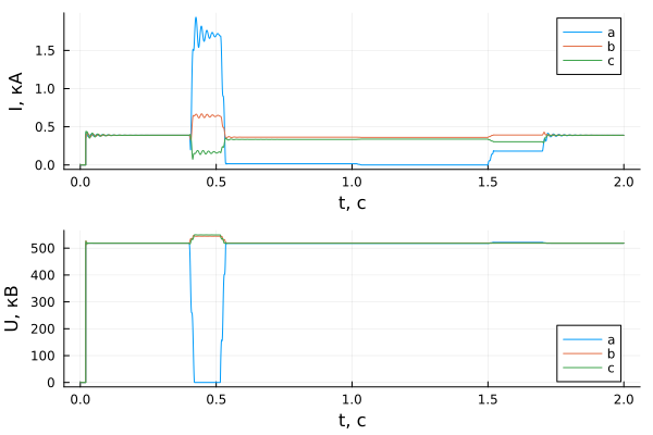
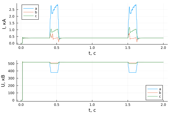
Checking the operation of the DZ and TNNP with an internal short circuit with a successful OAPV.
The sequence of modes:
- 0-0.5 s Normal load mode, preceding a short circuit
- 0.4 s Occurrence of a short circuit in the middle of the overhead
line - 0.5 s Disconnection of phase A of the line from both sides, A shockless pause (1.5 s) - 1 s Short circuit disappearance
- 1.5 s Activation of phase A (OAPV) from the side of PS A
- 1.7 s Activation of phase A lines from the side of PS B.
.png)
The model defines experience No. 17. For other experiments, it is necessary to change the short-circuit resistance in the short-circuit block and/or move it to the desired point.
model_name = "B2_17_20"
model_name in [m.name for m in engee.get_all_models()] ? engee.open(model_name) : engee.load( "$(@__DIR__)/$(model_name).engee");
results = Matrix{Any}(undef, 1, 4)
result = engee.run(model_name);
results[1, 1] = stack(collect(result["I1_1"].value[:])[!,:value])';
results[1, 2] = stack(collect(result["I2_1"].value[:])[!,:value])';
results[1, 3] = stack(collect(result["V1_1"].value[:])[!,:value])';
results[1, 4] = stack(collect(result["V2_1"].value[:])[!,:value])';
sim_time = collect(result["I1_1"].time[:])[!,:time];
Displaying results:
# measuring side, 1 - PS A, 2 -PS B
dir = 1;
gr()
p1 = plot(sim_time, results[1, dir], title = "Primary current, RMS", xlabel = "t, with", ylabel = "I, kA", label = ["a" "b" "c"])
p2 = plot(sim_time, results[1, dir+2], title = "Line voltage, RMS", xlabel = "t, with", ylabel = "U, kV", label = ["ab" "bc" "ca"])
plot(p1, p2, layout=(2,1))
Experiments 21-24
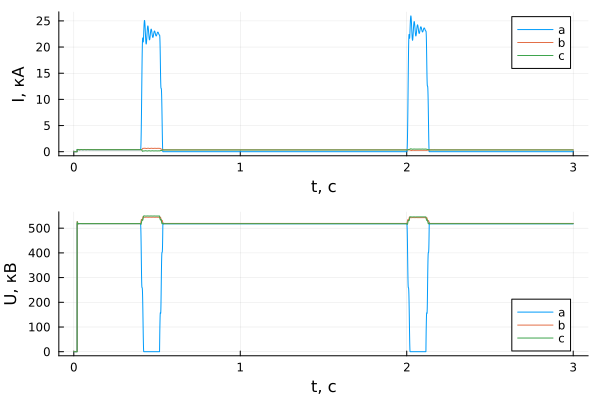
Checking the operation of the DZ and TNNP with an internal short circuit with an unsuccessful OAPV.
The sequence of modes:
- 0-0.4 s Normal load mode, preceding short circuit.
- 0.4 s Short circuit occurrence on the line
- 0.5 s Switching off phase A of the line with a short circuit on both sides, a shockless pause (1.5 s)
- 2 s Switching on phase A of the line from the side of the substation
- 2.1 s Disconnection of the line from the protection of PS A.
.png)
The model defines experience No. 21. For other experiments, it is necessary to change the short-circuit resistance in the short-circuit block and/or move it to the desired point.
model_name = "B2_21_24"
model_name in [m.name for m in engee.get_all_models()] ? engee.open(model_name) : engee.load( "$(@__DIR__)/$(model_name).engee");
results = Matrix{Any}(undef, 1, 4)
result = engee.run(model_name);
results[1, 1] = stack(collect(result["I1_1"].value[:])[!,:value])';
results[1, 2] = stack(collect(result["I2_1"].value[:])[!,:value])';
results[1, 3] = stack(collect(result["V1_1"].value[:])[!,:value])';
results[1, 4] = stack(collect(result["V2_1"].value[:])[!,:value])';
sim_time = collect(result["I1_1"].time[:])[!,:time];
Displaying results:
# measuring side, 1 - PS A, 2 -PS B
dir = 1
gr()
p1 = plot(sim_time, results[1, dir], title = "Primary current, RMS", xlabel = "t, with", ylabel = "I, kA", label = ["a" "b" "c"])
p2 = plot(sim_time, results[1, dir+2], title = "Line voltage, RMS", xlabel = "t, with", ylabel = "U, kV", label = ["ab" "bc" "ca"])
plot(p1, p2, layout=(2,1))
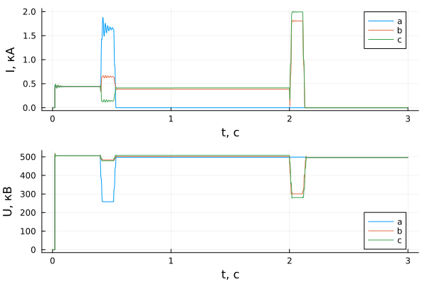
Experiments 25-30
Stable intermittent short circuit in the OAPV cycle.
The sequence of modes:
- 0-0.4 s Normal load mode.
- 0.4 s Short circuit occurrence.
- 0.5 s Disconnection of phase A of the line.
- 1 s The disappearance of the short circuit To (1)A0. Shockless pause (1.5 s).
- 2 with the inclusion of phase A of the line from the side of PS A and the occurrence of a short circuit of the phases of the sun.
- 2.1 with short circuit protection shutdown
.png)
The model has experience number 25. To carry out other experiments, it is necessary to change the resistance of the switches in the K1 subsystem. To change the short-circuit point, move the short-circuit block to the middle of the line.
model_name = "B2_25_30"
model_name in [m.name for m in engee.get_all_models()] ? engee.open(model_name) : engee.load( "$(@__DIR__)/$(model_name).engee");
results = Matrix{Any}(undef, 1, 4)
result = engee.run(model_name);
results[1, 1] = stack(collect(result["I1_1"].value[:])[!,:value])';
results[1, 2] = stack(collect(result["I2_1"].value[:])[!,:value])';
results[1, 3] = stack(collect(result["V1_1"].value[:])[!,:value])';
results[1, 4] = stack(collect(result["V2_1"].value[:])[!,:value])';
sim_time =  collect(result["I1_1"].time[:])[!,:time];
Displaying results:
# measuring side, 1 - PS A, 2 -PS B
dir = 2
gr()
p1 = plot(sim_time, results[1, dir], title = "Primary current, RMS", xlabel = "t, with", ylabel = "I, kA", label = ["a" "b" "c"])
p2 = plot(sim_time, results[1, dir+2], title = "Line voltage, RMS", xlabel = "t, with", ylabel = "U, kV", label = ["ab" "bc" "ca"])
plot(p1, p2, layout=(2,1))
Experience 31
Checking the operation of the DZ and TNNP with external short circuits with unsuccessful TAPV with TT saturation.
Test conditions:
- KZ location: point K4
- Type of short circuit: K(1)A0
- Transient resistance at the short circuit location: 0
The sequence of modes:
- 0-0.4 s Normal load mode.
- 0.4 s Short circuit occurrence.
- 0.5 s Disconnection of the damaged line.
- 1.5 s APV from the side of PS B (1 s).
- 1.6 s Disconnection of the damaged line.
model_name = "B2_31"
model_name in [m.name for m in engee.get_all_models()] ? engee.open(model_name) : engee.load( "$(@__DIR__)/$(model_name).engee");
results = Matrix{Any}(undef, 1, 4)
result = engee.run(model_name);
results[1, 1] = stack(collect(result["I1_1"].value[:])[!,:value])';
results[1, 2] = stack(collect(result["I2_1"].value[:])[!,:value])';
results[1, 3] = stack(collect(result["V1_1"].value[:])[!,:value])';
results[1, 4] = stack(collect(result["V2_1"].value[:])[!,:value])';
sim_time =  collect(result["I1_1"].time[:])[!,:time];
Displaying results:
# measuring side, 1 - PS A, 2 -PS B
dir = 1
gr()
p1 = plot(sim_time, results[1, dir], title = "Primary current, RMS", xlabel = "t, with", ylabel = "I, kA", label = ["a" "b" "c"])
p2 = plot(sim_time, results[1, dir+2], title = "Line voltage, RMS", xlabel = "t, with", ylabel = "U, kV", label = ["ab" "bc" "ca"])
plot(p1, p2, layout=(2,1))
Experiments 32-35
Swing with the swing center on the A-B line.
Test conditions:
- Swing center: on the A-B line.
- Swing frequency: 1 Hz and increase to failure of the swing lock.
.png)
The model has experience number 32. For other experiments, it is necessary to change the amplitude and frequency parameters of the "Sine function" block from the "Frequency" subsystem. For experiment No. 32, the EMF swing angle at PS B is set to ± 180° from the set mode. From 0 to 0.5 seconds, the system operates in steady state, and from 0.5 seconds, the frequency begins to change. The amplitude should be increased in proportion to the swing frequency.
model_name = "B2_32_35"
model_name in [m.name for m in engee.get_all_models()] ? engee.open(model_name) : engee.load( "$(@__DIR__)/$(model_name).engee");
results = Matrix{Any}(undef, 1, 4)
result = engee.run(model_name);
results[1, 1] = stack(collect(result["I1_1"].value[:])[!,:value])';
results[1, 2] = stack(collect(result["I2_1"].value[:])[!,:value])';
results[1, 3] = stack(collect(result["Zab_1"].value[:])[!,:value]);
results[1, 4] = stack(collect(result["Zab_2"].value[:])[!,:value]);
sim_time =  collect(result["I1_1"].time[:])[!,:time];
Displaying results:
# measuring side, 1 - PS A, 2 -PS B
dir = 1
gr()
p1 = plot(sim_time, results[1, dir], title = "Primary current, RMS", xlabel = "t, with", ylabel = "I, kA", label = ["a" "b" "c"])
p2 = plot(sim_time, results[1, dir+2], title = "Resistance", xlabel = "t, with", ylabel = "Zab, Om", ylims = (0, 2000), legend = false)
plot(p1, p2, layout=(2,1))
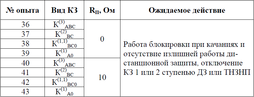
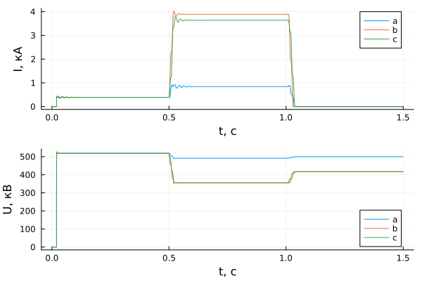
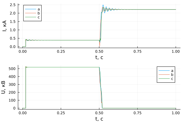
Experiments 36-43
Swing with the swing center on the A-B line and short circuit in the protection area.
Test conditions:
- Swing center: on line A-B, 60% of the line length from point A.
- Swing frequency: 2 Hz
- KZ location: 60% of the line from PS A.
- Type of short circuit: K(3)ABC, K(2)BC, K(1,1)BC0, K(1)A0
- The resistance at the short-circuit point is 0 and 10 ohms.
.png)
The model defines experience No. 36. For other experiments, it is necessary to change the type of short circuit and the transient resistance in the short circuit block. For experiment No. 36, the EMF swing angle at PS B is set to ± 180° from the set mode. From 0 to 0.5 seconds, the system operates in steady state, from 0.5 seconds the frequency begins to change, at 1.125 seconds a short circuit occurs at point K7.
model_name = "B2_36_43"
model_name in [m.name for m in engee.get_all_models()] ? engee.open(model_name) : engee.load( "$(@__DIR__)/$(model_name).engee");
results = Matrix{Any}(undef, 1, 4)
result = engee.run(model_name);
results[1, 1] = stack(collect(result["I1_1"].value[:])[!,:value])';
results[1, 2] = stack(collect(result["I2_1"].value[:])[!,:value])';
results[1, 3] = stack(collect(result["Zab_1"].value[:])[!,:value]);
results[1, 4] = stack(collect(result["Zab_2"].value[:])[!,:value]);
sim_time =  collect(result["I1_1"].time[:])[!,:time];
Displaying results:
# measuring side, 1 - PS A, 2 -PS B
dir = 1
gr()
p1 = plot(sim_time, results[1, dir], title = "Primary current, RMS", xlabel = "t, with", ylabel = "I, kA", label = ["a" "b" "c"])
p2 = plot(sim_time, results[1, dir+2], title = "Resistance", xlabel = "t, with", ylabel = "Zab, Om", ylims = (0, 2000), legend = false)
plot(p1, p2, layout=(2,1))
Experience 44
An external short circuit on a parallel line that turns into an internal one.
Test conditions:
- Type of short circuit: External to (3)ABC, turning into internal.
- KZ location: point K5 with transition to point K1.
- Line load: normal mode (Table 2).
- Angle of occurrence of short circuit: 0°.
- The transient resistance at the short-circuit point is 0 ohms.
The sequence of modes:
- Short circuit of phases ABC on a parallel line from the side of PS A.
- After 60 ms, the short circuit switches to the protected line at point K1.
The sequence of events:
- 0.5 s 3f short circuit at point K5 (the voltage angle of phase A is zero).
- 0.56 s 3f short circuit occurs at point K1 (short circuit at point K5 does not disappear).
- 0.6 s short circuit shutdown at point K5.
- 0.66 s short circuit shutdown at point K1.
.png)
model_name = "B2_44"
model_name in [m.name for m in engee.get_all_models()] ? engee.open(model_name) : engee.load( "$(@__DIR__)/$(model_name).engee");
results = Matrix{Any}(undef, 1, 4)
result = engee.run(model_name);
results[1, 1] = stack(collect(result["I1_1"].value[:])[!,:value])';
results[1, 2] = stack(collect(result["I2_1"].value[:])[!,:value])';
results[1, 3] = stack(collect(result["V1_1"].value[:])[!,:value])';
results[1, 4] = stack(collect(result["V2_1"].value[:])[!,:value])';
sim_time = collect(result["I1_1"].time[:])[!,:time];
Displaying results:
# measuring side, 1 - PS A, 2 -PS B
dir = 1
gr()
p1 = plot(sim_time, results[1, dir], title = "Primary current, RMS", xlabel = "t, with", ylabel = "I, kA", label = ["a" "b" "c"])
p2 = plot(sim_time, results[1, dir+2], title = "Line voltage, RMS", xlabel = "t, with", ylabel = "U, kV", label = ["ab" "bc" "ca"])
plot(p1, p2, layout=(2,1))
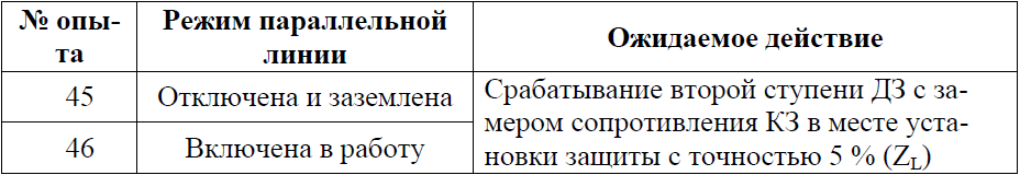
Experiments 45-46
The effect of the mutual induction of the parallel line on the operation of the DZ.
Test conditions:
- Normal mode.
- KZ location: point K2.
- Resistance at the short circuit location: 0 Ohms.
- Short circuit type: K(1)A0
- a) The parallel line is disconnected and grounded.
- b) Parallel line in operation.
.png)
The model defines experience No. 45. To carry out experiment No. 46, it is necessary to turn on switches Q3 and Q4, disconnect the grounding knives.
model_name = "B2_45_46"
model_name in [m.name for m in engee.get_all_models()] ? engee.open(model_name) : engee.load( "$(@__DIR__)/$(model_name).engee");
results = Matrix{Any}(undef, 1, 4);
result = engee.run(model_name);
results[1, 1] = stack(collect(result["I1_1"].value[:])[!,:value])';
results[1, 2] = stack(collect(result["I2_1"].value[:])[!,:value])';
results[1, 3] = stack(collect(result["Zab_1"].value[:])[!,:value]);
results[1, 4] = stack(collect(result["Zab_2"].value[:])[!,:value]);
sim_time = collect(result["I1_1"].time[:])[!,:time];
Displaying results:
# measuring side, 1 - PS A, 2 -PS B
dir = 1
gr()
p1 = plot(sim_time, results[1, dir], title = "Primary current, RMS", xlabel = "t, with", ylabel = "I, kA", label = ["a" "b" "c"])
p2 = plot(sim_time, results[1, dir+2], title = "Resistance", xlabel = "t, with", ylabel = "Zab, Om", ylims = (0, 500), legend = false)
plot(p1, p2, layout=(2,1))