Autonomous hybrid power plant: diesel + solar+ storage
This example shows a model of an autonomous diesel-solar power plant with an energy storage system based on supercapacitors. The model is used for:
- Checking the SNE control algorithm
- Selecting the parameters of the solar power plant
- Selection of power, energy intensity, type of storage devices
- Calculating economic efficiency from fuel economy
- Choosing the optimal number of units and the size of the installed capacity of the DSU
Introduction
Digital modeling plays a key role in the development and testing of SNE control algorithms, allowing us to study the operating modes of power systems and assess the impact of storage devices on sustainability and efficiency without conducting field experiments.
One of the promising areas of application of SNES is autonomous hybrid power plants (ASES), which are widely used for power supply to remote facilities, including oil and gas producing enterprises. Such power systems are characterized by a lack of communication with the UES, a rapidly changing nature of the load, as well as increased requirements for the reliability of power supply.
When designing ASUE, the DSU capacity is usually selected based on the maximum load, as a result of which the installed capacity utilization factor (KIUM) turns out to be low. This leads to the operation of diesel installations in uneconomical modes, accompanied by increased fuel consumption, accelerated wear of equipment, activation of technological protections and deterioration of electricity quality. In addition, to ensure the reliability of power supply, it is often necessary to overestimate the installed capacity of generating units, which reduces the economic efficiency of ASUE.
The use of SNES as part of the ASUE makes it possible to smooth out sudden load changes, improve the quality of frequency and voltage regulation, ensure the operation of generators near economical modes and reduce the requirements for the installed capacity of traditional sources. In this regard, the development and research of a demo model of ASUE with SNE using digital modeling is an urgent task for substantiating control algorithms and system parameters.
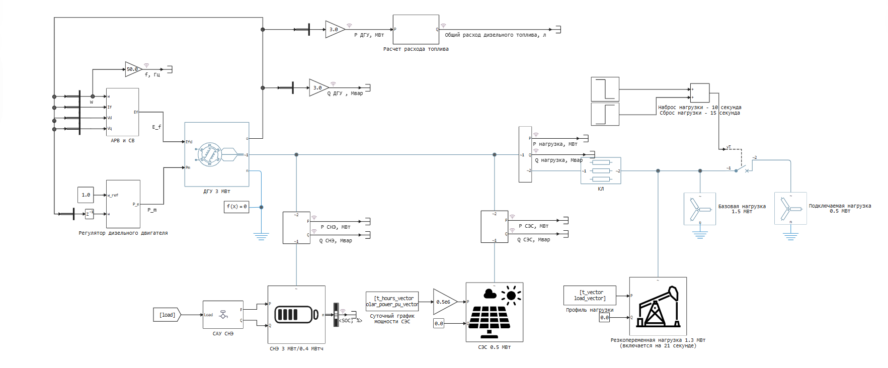
Description of the model
The 10.5 kV model includes:
· Diesel generator set (DGU) with ARV SD and APC with a capacity of 3 MW;
· Solar power plant (SES) with a capacity of 0.5 MW, without regulators;
· SNES with a capacity of 3 MW and an energy capacity of 400 kWh with an algorithm for smoothing load power surges;
· Cable line for connection of generating equipment and load;
· 3.3 MW load (base power – 1.5 MW, variable – 0.5 MW, variable -1.3 MW).
Export files for the model
For the model to work, we export the necessary dependencies from the file system.:
using JLD2
@load "load_profile.jld2"; # graph of alternating load, W(s)
@load "charging_curve.jld2"; # dependence of the available power of the supercapacitor on the charge, W(%)
@load "fuel_consumption_curve.jld2"; # dependence of fuel consumption on load l/h(MW)
@load "specific_fuel_consumption.jld2"; # dependence of specific fuel consumption on load k*kWh (O.E.)
@load "solar_profile_pu.jld2"; # daily schedule of SES capacity, O.E.(c)
Graphs of exported dependencies
using Plots
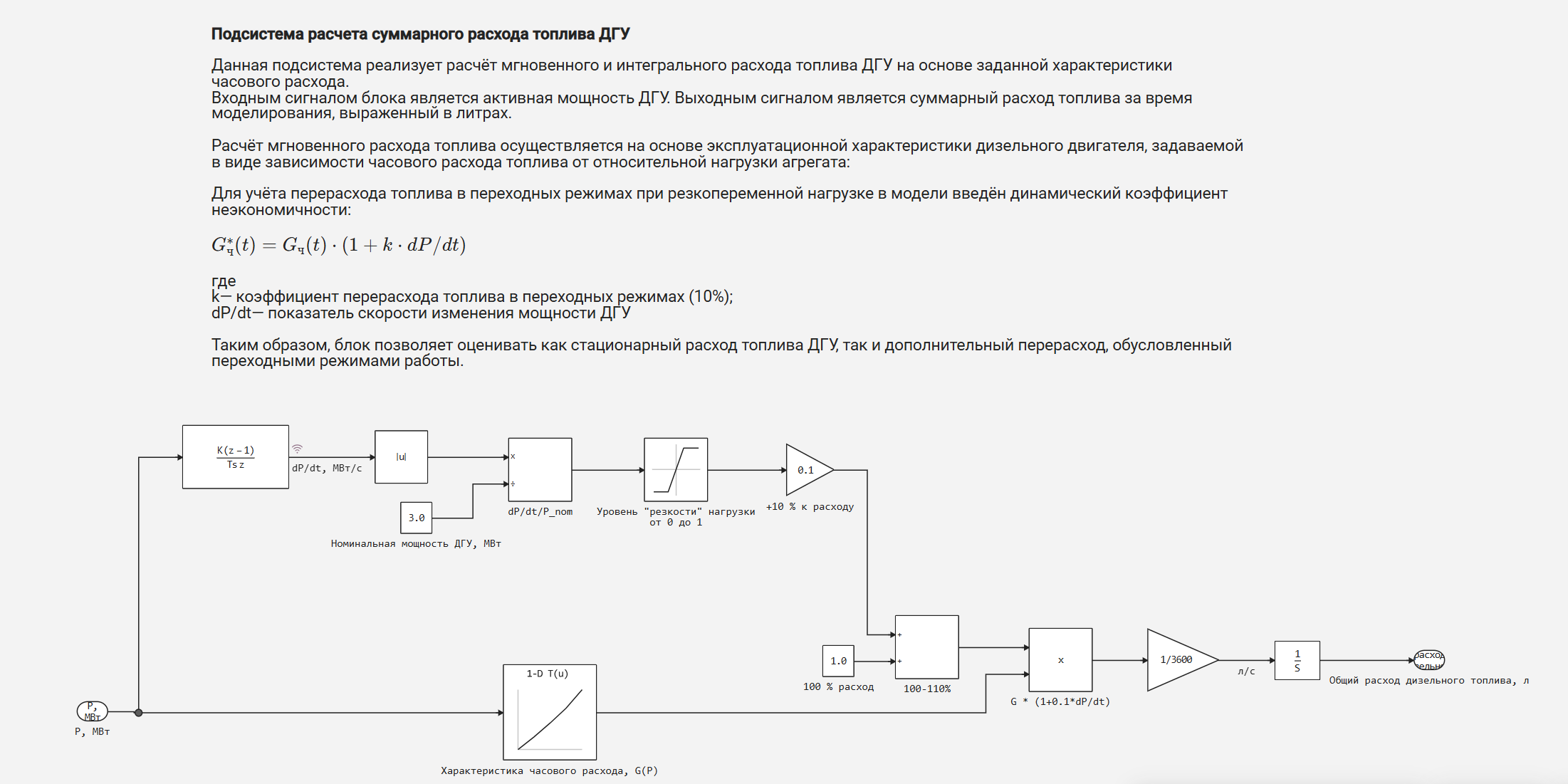
Hourly fuel consumption of the DGU. This relationship is used in the model to calculate the current fuel consumption and the total amount of fuel consumed over the entire duration of the simulation.
plot(procent_of_load_vector, G_vector,
    linewidth=2,
    linecolor=:black,
    marker=:circle,
    markersize=5,
    markercolor=:white,
    markerstrokecolor=:black,
    markerstrokewidth=1,
    xlabel="Load, %",
    ylabel="Consumption, l/h",
    grid=true,
    gridalpha=0.2,
    gridstyle=:dash,
    framestyle=:box,
    size=(800, 400),
    dpi=150,
    legend=false,
    background_color=:white
)
Fragment of the load diagram of the lifting and transport mechanism. Used in the model to set the profile of the variable load.
plot( t_vector[1:5000], load_vector[1:5000]./1e6,
    linewidth=2,
    linecolor=:black,
    # marker=:circle,
    markersize=5,
    markercolor=:white,
    markerstrokecolor=:black,
    markerstrokewidth=1,
    xlabel="Time, from",
    ylabel="Load, MW",
    grid=true,
    gridalpha=0.2,
    # gridstyle=:dash,
    framestyle=:box,
    size=(800, 400),
    dpi=150,
    legend=false,
    background_color=:white,
)
hline!([0.33], # average power value
    linecolor=:red,
    linewidth=2,
    linestyle=:dash,
)
The average value of the power of the alternating load:
average_power = sum(load_vector) / length(load_vector)/1e6
Maximum power value of the alternating load:
max_power=maximum(load_vector)/1e6
The dependence of specific fuel consumption on the load for a 3 MW CSU. The graph clearly shows that at low load, significantly more fuel is required to generate 1 kWh of electricity. This dependence is not used in the model, but demonstrates the problem of isolated power systems, where most often generating units operate at a low load of 10 to 40% (as previously calculated, the average load of the lifting and transport mechanism profile is only 0.33 MW, with a maximum value of 1.3 MW)
plot(procent_of_load_vector, g_vector,
    linewidth=2,
    linecolor=:black,
    marker=:circle,
    markersize=5,
    markercolor=:white,
    markerstrokecolor=:black,
    markerstrokewidth=1,
    xlabel="Load, %",
    ylabel="Consumption, g/kWh",
    grid=true,
    gridalpha=0.2,
    gridstyle=:dash,
    framestyle=:box,
    size=(800, 400),
    dpi=150,
    legend=false,
    background_color=:white
)

# Shaded area up to 50% load
vspan!(0, 50, fillalpha=0.08, linealpha=0)

# Vertical border 50 %
vline!([50], linestyle=:dash, linewidth=1)

# Text annotation
annotate!(25, maximum(g_vector)*0.95, text("The zone of increased fuel consumption", 9, :black))
annotate!(52, minimum(g_vector)*1.05, text("", 8, :black))
Available power of supercapacitors depending on the charge. The curve is set in the SNE model to simulate the characteristics of a real storage device. This curve can be obtained in a separate auxiliary Engee model during the simulation by applying voltage to the supercapacitor units, lithium-ion batteries, and other available types of storage devices from the library. In this example, the process of obtaining a curve is not considered and is exported as a finished file.
plot(SOC_vector./1e6, P_vector./1e6,
    linewidth=2,
    linecolor=:black,
    markercolor=:white,
    markerstrokecolor=:black,
    markerstrokewidth=1,
    xlabel="Charge, %",
    ylabel="Available capacity of the SC, MW",
    grid=true,
    gridalpha=0.2,
    gridstyle=:dash,
    framestyle=:box,
    size=(800, 400),
    dpi=150,
    legend=false,
    background_color=:white
)
It follows from this relationship that the available power varies non-linearly. From here, you can set the minimum and maximum SNE charge from 10 to 90%.
Daily schedule of SES capacity.
plot(t_hours_vector./3600, solar_power_pu_vector,
    linewidth=2,
    linecolor=:black,
    marker=:circle,
    markersize=5,
    markercolor=:white,
    markerstrokecolor=:black,
    markerstrokewidth=1,
    xlabel="Time, h",
    ylabel="SES capacity, O.E.",
    grid=true,
    gridalpha=0.2,
    gridstyle=:dash,
    framestyle=:box,
    size=(800, 400),
    dpi=150,
    legend=false,
    background_color=:white
)
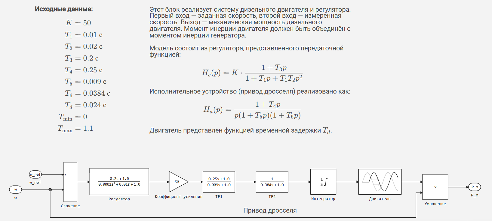
Description of the DSU model
The DSU model is presented in the form of a generator in phase координатах , diesel engine models with speed control, ARV-M and возбудителя:
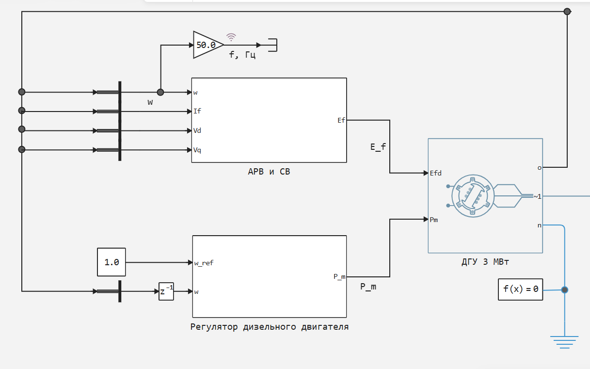
The model of the engine and speed controller is shown below:
Subsystem for calculating total fuel consumption
Description of the SNE model
The generalized block diagram of the SNE as part of the power system is as follows:
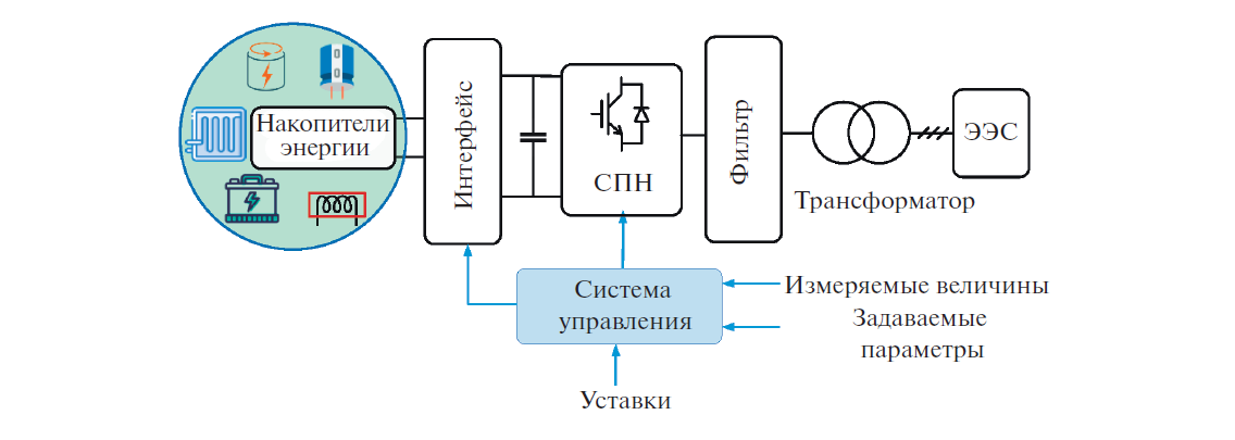
A three-phase bidirectional power voltage converter (CNV) is one of the main elements in the SNE connection scheme to the power system. The principle of sinusoidal pulse width modulation is mainly used to control the keys. We have considered detailed SNE models in the examples. <https://engee.com/community/ru/catalogs/projects/trekhfaznyi-invertor-s-sistemoi-upravleniia-na-kpm-ritm > and <https://engee.com/community/ru/catalogs/projects/istochnik-bespereboinogo-pitaniia >. In addition, we also talked about the techniques of modeling converters in https://engee.com/community/ru/catalogs/projects/sravnenie-tekhnik-modelirovaniia-ac-dc-preobrazovatelei.
In our example, to reduce the calculation time in the study of long-term electromechanical transients, the SNE model was developed on the basis of a three-phase controlled power source without using detailed models of a power converter and supercapacitors (the energy storage subsystem is determined by its external characteristic). This solution allows you to increase the calculation step by several orders of magnitude, which in turn reduces the requirements for computing power, and also allows you to calculate electromechanical transients lasting several hours.
The presented SNE model consists of a directional (basic blocks of mathematics) and a non-directional (physical model) part. The directional part is a model of directional blocks of basic mathematics, where two signals are generated: active and reactive power for the dynamic load unit. Before transmitting power signals to the physical module, there is a minus sign, so the dynamic load unit will play the role of a power source. Below is a block diagram of the SNE model, designed to calculate electromechanical transients and study control algorithms in the power system.
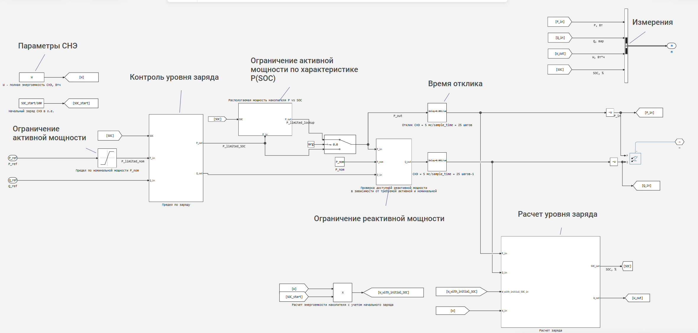
The SNE model includes the following functional blocks:
1. The block for setting SNE parameters.
In this block, the main nominal parameters of the drive are set:
– the total energy consumption of the SNE W, Wh;
– the initial charge level of the SOC_start, %;
2. Limitation of the active power according to the nominal value.
The input value for active power P_ref is limited by the nominal value P_nom. This allows you to take into account the limitations of the converter equipment in terms of the maximum allowable output and power consumption.
3. Charge level control (SOC).
The unit implements active power limits depending on the current charge level of the drive. When the SOC limits (minimum and maximum) are reached, the available discharge or charge power is automatically reduced.
Additionally, a limitation is implemented on the characteristic of the supercapacitor P(SOC), set by a tabular dependence, which allows for a decrease in available power at a low charge level.
4. Limitation of reactive power.
The permissible reactive power Q is checked depending on the current active power and the rated power. This ensures that the full capacity limits are met.
5. The model of the dynamics of the SNE response.
The dynamics of changes in active and reactive power is described by a delay with a given response time.
6. Calculation of the charge level (SOC).
The charge level is calculated based on the current active and reactive power of the SNE and the initial charge value.
7. Formation of measured values.
The following signals are generated at the output of the model:
– active power P, W;
– reactive power Q, var;
– current SOC charge level, %;
– current energy consumption of the drive W, W·h.
SNE control algorithm for load power smoothing
The SNE control algorithm for frequency control in an autonomous power system performs load surge/discharge smoothing.
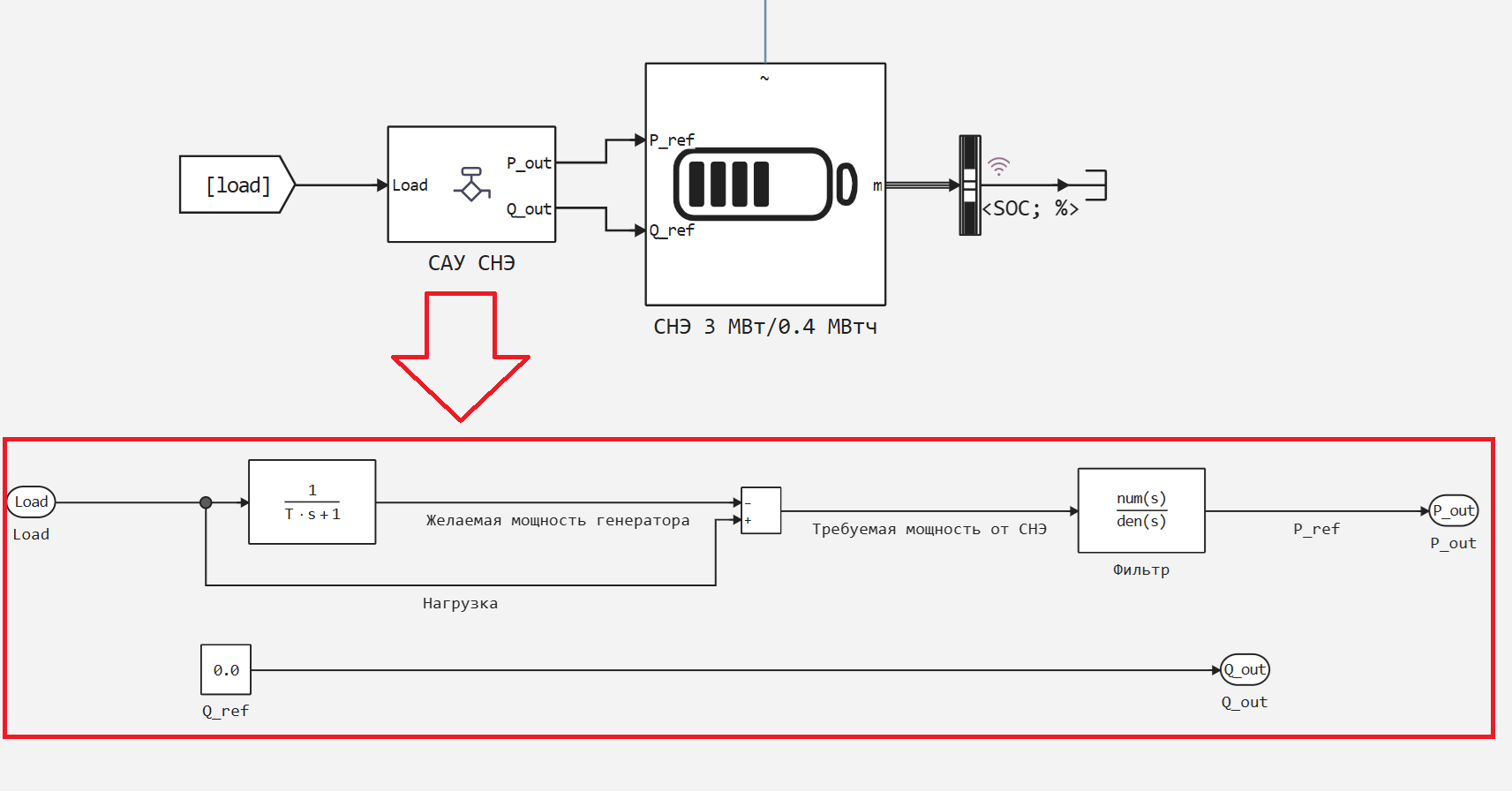
A load power signal is applied to the input of the adder. Next, this signal is duplicated via one of the control channels. One of the signals passes through an aperiodic link of the first order, in which the time constant T is set, which affects the smooth transmission of load power from the SNE to the DSU. A smooth load signal is obtained at the output of the aperiodic link. When adding the load signal and the smoothed load signal, a signal of the required power from the SNE is obtained. This signal can be either positive or negative. A positive value corresponds to power output (discharge), a negative value corresponds to power consumption (charge).
Simulation results
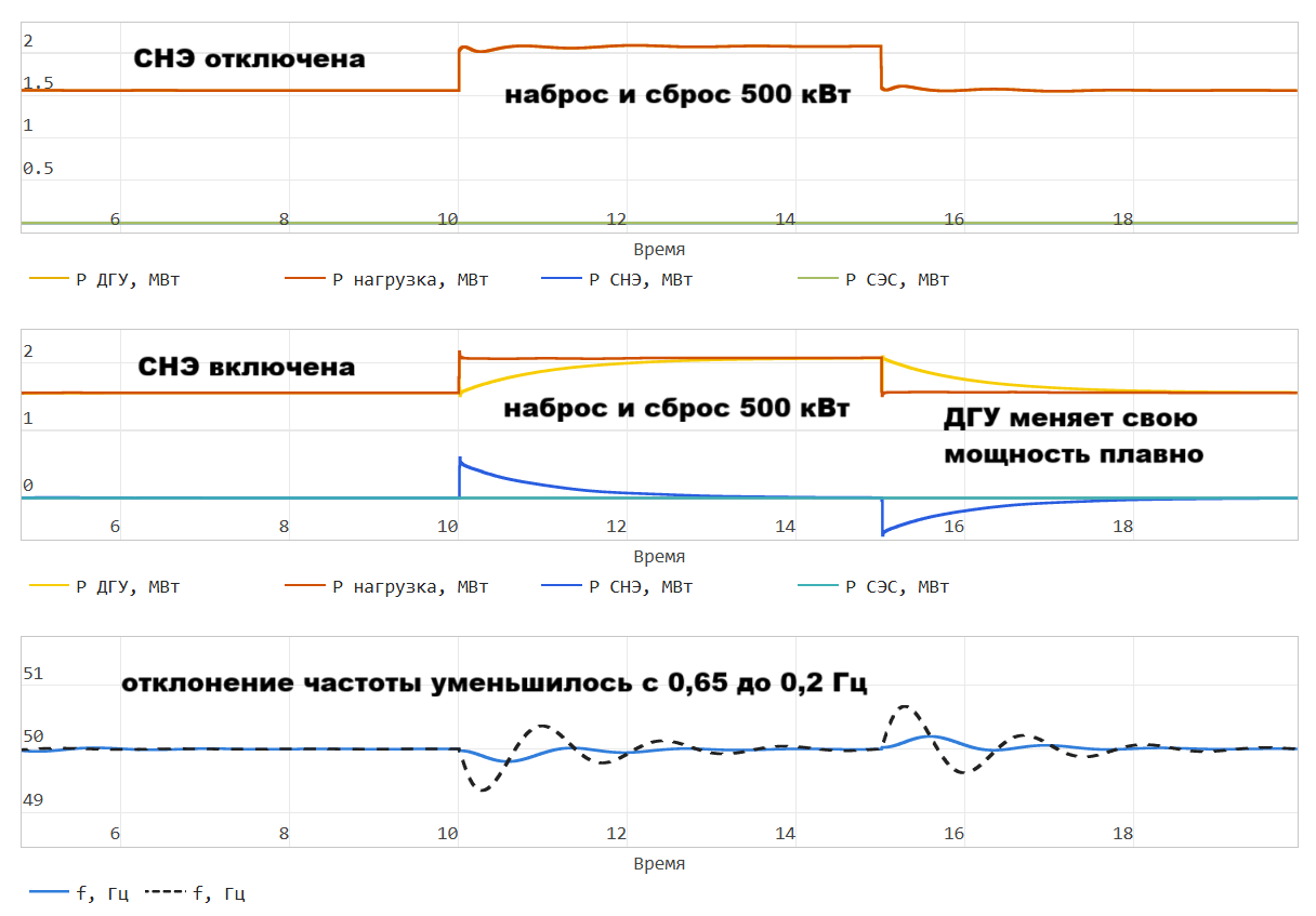
Experience 1 and 2. Loading and unloading 0.5 MW of load on the DSU with the SNE on and off. The duration of the simulation is 20 seconds. The time constant of the algorithm is 1 second.
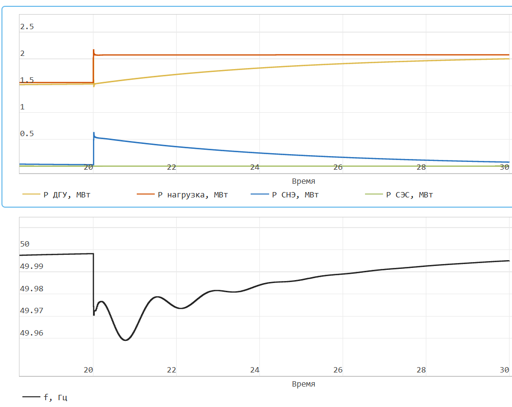
Experience 3. Applying 0.5 MW of load to the DSU with the SNE turned on. The duration of the simulation is 30 seconds. The time constant of the algorithm is 5 seconds.
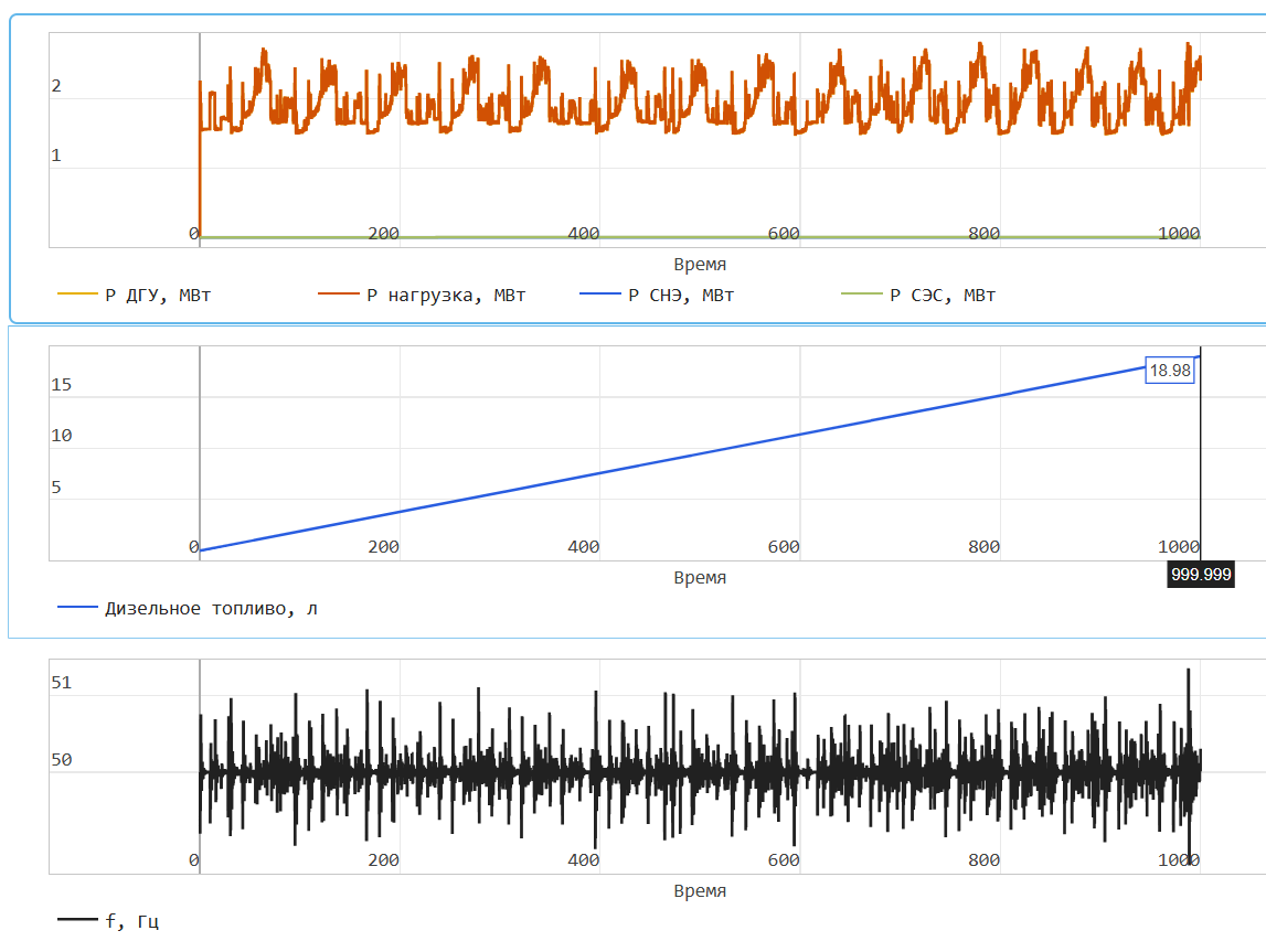
Experience 4. DSU work on a sharply alternating load of a lifting mechanism without SES and without SNE. The duration of the simulation is 1000 seconds.
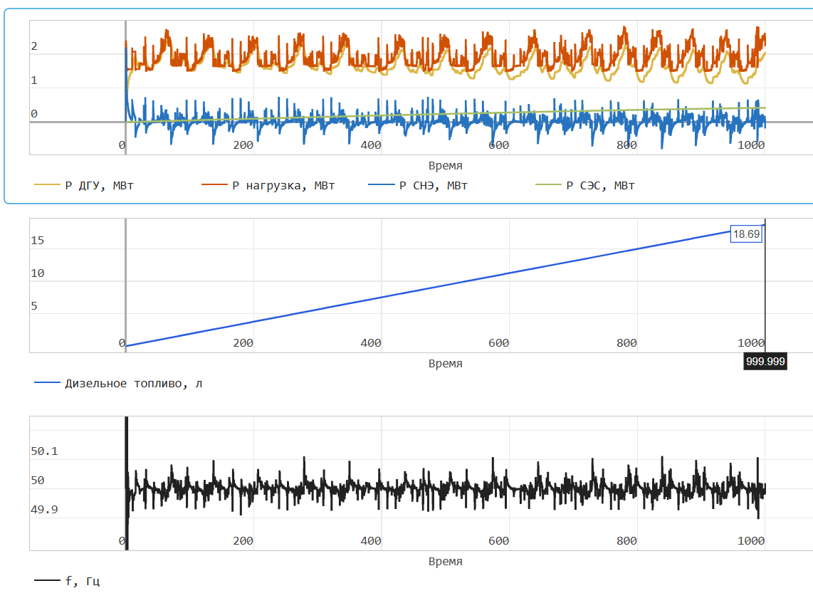
Experience 5. DSU work on a sharply alternating load of a lifting mechanism with SES and SNE. The duration of the simulation is 1000 seconds. The SES capacity increases from 0 to 0.42 MW during the simulation. The SNE works according to an algorithm for smoothing load power surges.
Conclusions
- This project shows an ASUE model for calculating electromechanical transients. The model is designed for calculating modes, transients, and stability of power systems that include DGS, SNES, and SES, as well as for developing and testing SNE control algorithms that increase the controllability and reliability of power systems.
- A simplified SNE model has been developed for calculating long-term electromechanical transients.
- An alogrithm of SNE control is proposed. Based on experiments No. 1 and No. 2, it can be said that the use of the SNE control algorithm to smooth load surges/drops reduced the frequency deviation from 0.65 Hz to 0.2 Hz when applying 0.5 MW of load with a time constant of the algorithm equal to 1 second. In experiment 3, when the time constant of the smoothing algorithm was increased to 5 seconds, the frequency deviation at 0.5 MW decreased to 0.05 Hz. Based on experiments No. 4 and No. 5, when ASUE was operating with SES and SNE turned on, diesel fuel consumption decreased from 19 to 18.7 liters and the quality of frequency control increased (the maximum deviation decreased 10-fold from 1 Hz to 0.1 Hz).