B3 Program and test procedure for remote protection (DZ) for lines with voltage up to 35 kV
In this example, a test network model is implemented to perform DZ functional tests for lines with a voltage of up to 35 kV from Appendix B3 STO 56947007-29.120.70.241-2017. Technical requirements for RPA microprocessor devices. This example contains 9 models named B3_X.engee, where X is the number or range of experiment numbers. The model has been adapted and tested for launch at KPM RHYTHM. For more information about using KPM RHYTHM, see the examples KPM RHYTHM: Quick Start and KPM RHYTHM: Real-time operation. Examples of experiments are made to demonstrate without connecting real equipment, you need to connect it yourself. To connect the RPA terminal, you need to add DAC blocks and digital inputs/outputs from the RHYTHM block library to the model, then connect the terminal to the RHYTHM KPM. The scheme of the simulated network:
System 1:
EMF – 38.5 kV
The resistance of the direct sequence is 0.286 + j2.7 ohms
The EMF phase angle is 0°
System 2:
EMF – 37.2 kV
The resistance of the direct sequence is 0.456 + j4.3 ohms
The EMF phase angle is -5°
VL13:
Length — 16 km
Wire brand — AC-95
The resistance is straight. posl. — 4,816 + j6,736 ohms
Resistance zero. pos. — 7,224 + j20,208 ohms
Large capacity. OZZ current — 1.6 A
VL32:
Length — 12 km
The wire brand is AC-95
The resistance is straight. posl. — 3,612 + j5.052 ohms
Resistance zero. pos. — 5,418 + j15,156 ohms
Large capacity. OZZ current — 1.2 A
VL12 (PS1-PS4):
Length — 6 km
Wire brand — AC-120
The resistance is straight. posl. — 1,464 + j2,484 ohms
Resistance zero. pos. — 2,196 + j7,452 ohms
Large capacity. OZZ current — 0.6 A
VL12 (PS4-PS2):
Length — 8 km
Wire brand — AC-120
The resistance is straight. posl. — 1,952 + j3,312 ohms
Resistance zero. pos. — 2.928 + j9.936 ohms
Large capacity. OZZ current — 0.8 A
Measuring current transformers:
TFZM-35B-1
ct = 300 / 5 A
Z2ohm = 0.8 ohms (cos φ = 0.8)
K10 = 30
Qmh = 19.2 cm2
Lcp = 0.82 m
W_1 = 4
W2 = 239
R2obm = 0.45 ohms
Checking the first DZ zone
The zone of operation of the first stage of the remote control with a three-phase short circuit is determined by simulating a short circuit on the protected line. From the RHYTHM installation, currents and voltages of the VL13 line are supplied to the terminal. The result is recorded: 95% of the setpoint – the first stage of the DZ is triggered, 105% of the setpoint – the first stage of the DZ is not triggered.
Test conditions:
- K(3) at a distance equal to 95% of the first zone.
- To (3) at a distance equal to 105% of the first zone.
In the VL13 model, it is divided in half (two segments of 8 km each). To determine the zone of operation of the first stage of the DZ, it is necessary to change the length of the segments in accordance with the terminal setting.
model_name = "B3_first_zone"
model_name in [m.name for m in engee.get_all_models()] ? engee.open(model_name) : engee.load( "$(@__DIR__)/$(model_name).engee");
results = Vector{Any}(undef, 3)
result = engee.run(model_name);
results[1] = stack(collect(result["I1"].value[:])[!,:value])';
results[2] = stack(collect(result["I2"].value[:])[!,:value])';
results[3] = stack(collect(result["V1"].value[:])[!,:value])';
sim_time = collect(result["I1"].time[:])[!,:time];
Displaying results:
gr()
p1 = plot(sim_time, results[1], title = "TT1",xlabel = "t, with", ylabel = "I, kA", label = ["a" "b" "c"])
p2 = plot(sim_time, results[2], title = "TT2",xlabel = "t, with", ylabel = "I, kA", label = ["a" "b" "c"])
p3 = plot(sim_time, results[3], title = "Line voltage, RMS (PS1)", xlabel = "t, with", ylabel = "U, kV", label = ["ab" "bc" "ca"])
plot(p1, p2, p3, layout=(3,1), size = (800, 600))
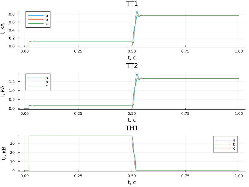
Experiments 1-2
Checking the operation of the remote control for various types of internal short circuits.
Test conditions:
- KZ location: point: Q1.
- Type of short circuit: K (2)Sun, K (3)
Experiment parameters:
Experiment No. 1 is set in the model. To conduct experiment No. 2, it is necessary to change the view of the short circuit and move the short circuit block to point K3.
model_name = "B3_1_2"
model_name in [m.name for m in engee.get_all_models()] ? engee.open(model_name) : engee.load( "$(@__DIR__)/$(model_name).engee");
results = Vector{Any}(undef, 3)
result = engee.run(model_name);
results[1] = stack(collect(result["I1"].value[:])[!,:value])';
results[2] = stack(collect(result["I2"].value[:])[!,:value])';
results[3] = stack(collect(result["V1"].value[:])[!,:value])';
sim_time = collect(result["I1"].time[:])[!,:time];
Displaying results:
gr()
p1 = plot(sim_time, results[1], title = "TT1",xlabel = "t, with", ylabel = "I, kA", label = ["a" "b" "c"])
p2 = plot(sim_time, results[2], title = "TT2",xlabel = "t, with", ylabel = "I, kA", label = ["a" "b" "c"])
p3 = plot(sim_time, results[3], title = "Line voltage, RMS (PS1)", xlabel = "t, with", ylabel = "U, kV", label = ["ab" "bc" "ca"])
plot(p1, p2, p3, layout=(3,1), size = (800, 600))
Experiments 3-4
Checking the operation of the remote control by "memory" with external three-phase short circuits on the buses.
Test conditions:
- KZ location: point K4.
- Type of short circuit: K(3)ABC, K(2)BC
Experiment parameters:
.png)
Experience No. 3 is set in the model. To carry out experiment No. 4, you need to change the view in the KZ block.
model_name = "B3_3_4"
model_name in [m.name for m in engee.get_all_models()] ? engee.open(model_name) : engee.load( "$(@__DIR__)/$(model_name).engee");
results = Vector{Any}(undef, 3)
result = engee.run(model_name);
results[1] = stack(collect(result["I1"].value[:])[!,:value])';
results[2] = stack(collect(result["I2"].value[:])[!,:value])';
results[3] = stack(collect(result["V1"].value[:])[!,:value])';
sim_time = collect(result["I1"].time[:])[!,:time];
Displaying results:
gr()
p1 = plot(sim_time, results[1], title = "TT1",xlabel = "t, with", ylabel = "I, kA", label = ["a" "b" "c"])
p2 = plot(sim_time, results[2], title = "TT2",xlabel = "t, with", ylabel = "I, kA", label = ["a" "b" "c"])
p3 = plot(sim_time, results[3], title = "Line voltage, RMS (PS1)", xlabel = "t, with", ylabel = "U, kV", label = ["ab" "bc" "ca"])
plot(p1, p2, p3, layout=(3,1), size = (800, 600))
Experience 5-16
Checking the operation of the remote control on each overhead line in case of double earth faults.
Test conditions:
- Short circuit location and protection installation location: according to the table.
- Type of short circuit: K(1)A and K(1)B
.png)
Experience number 5 is set in the model. For other experiments, it is necessary to move the short circuit blocks to the required points and change the type of short circuit in the blocks.
model_name = "B3_5_16"
model_name in [m.name for m in engee.get_all_models()] ? engee.open(model_name) : engee.load( "$(@__DIR__)/$(model_name).engee");
results = Vector{Any}(undef, 3)
result = engee.run(model_name);
results[1] = stack(collect(result["I1"].value[:])[!,:value])';
results[2] = stack(collect(result["I2"].value[:])[!,:value])';
results[3] = stack(collect(result["V1"].value[:])[!,:value])';
sim_time = collect(result["I1"].time[:])[!,:time];
Displaying results:
gr()
p1 = plot(sim_time, results[1], title = "TT1",xlabel = "t, with", ylabel = "I, kA", label = ["a" "b" "c"])
p2 = plot(sim_time, results[2], title = "TT2",xlabel = "t, with", ylabel = "I, kA", label = ["a" "b" "c"])
p3 = plot(sim_time, results[3], title = "Line voltage, RMS (PS1)", xlabel = "t, with", ylabel = "U, kV", label = ["ab" "bc" "ca"])
plot(p1, p2, p3, layout=(3,1), size = (800, 600))
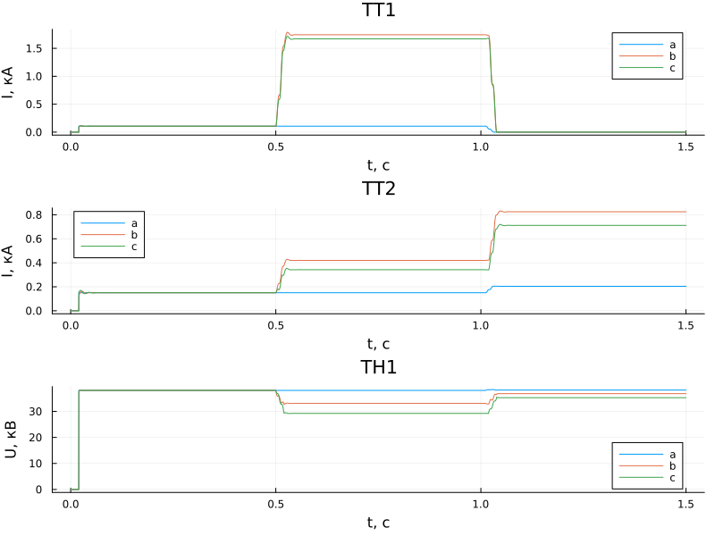
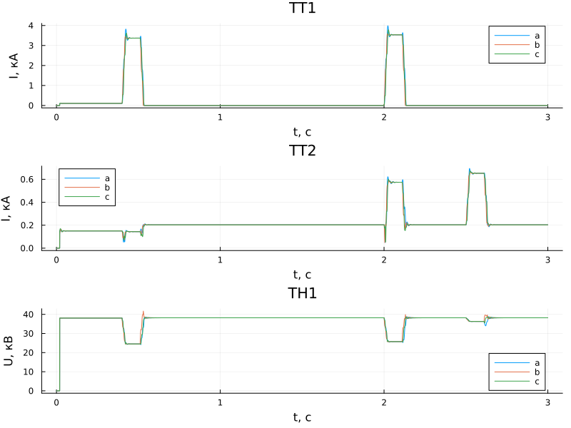
Experience 17-18
Checking the protection operation during an internal short circuit with a successful TAP.
Test conditions:
- KZ location: the middle of VL13 (point K6).
- Type of short circuit: K^(3)ABC, K(2)BC
The sequence of events:
- 0-0.4 s Normal load mode, preceding short circuit
- 0.4 s Occurrence of short circuit in the middle of the overhead line.
- 0.5 s Three-phase disconnection of the line with protections on both sides. Shockless pause (1.5 s)
- 1 s Short circuit disappearance
- 2 from the TAPB on the side of PS 1
- 2.5 s TAPV from the side of PS 3.
.png)
The model defines experience No. 17. To conduct experiment No. 18, it is necessary to change the type of short circuit in the short circuit block.
model_name = "B3_17_18"
model_name in [m.name for m in engee.get_all_models()] ? engee.open(model_name) : engee.load( "$(@__DIR__)/$(model_name).engee");
results = Vector{Any}(undef, 3)
result = engee.run(model_name);
results[1] = stack(collect(result["I1"].value[:])[!,:value])';
results[2] = stack(collect(result["I2"].value[:])[!,:value])';
results[3] = stack(collect(result["V1"].value[:])[!,:value])';
sim_time = collect(result["I1"].time[:])[!,:time];
Displaying results:
gr()
p1 = plot(sim_time, results[1], title = "TT1",xlabel = "t, with", ylabel = "I, kA", label = ["a" "b" "c"])
p2 = plot(sim_time, results[2], title = "TT2",xlabel = "t, with", ylabel = "I, kA", label = ["a" "b" "c"])
p3 = plot(sim_time, results[3], title = "Line voltage, RMS (PS1)", xlabel = "t, with", ylabel = "U, kV", label = ["ab" "bc" "ca"])
plot(p1, p2, p3, layout=(3,1), size = (800, 600))
Experiments 19-20
Checking the protection operation in case of an internal short circuit with an unsuccessful TAP.
Test conditions:
- KZ location: the middle of VL13 (point K6).
- Type of short circuit: K(3)ABC, K(2)BC
The sequence of events:
- 0-0.4 s Normal load mode, preceding short circuit
- 0.4 s Occurrence of short circuit in the middle of the overhead line.
- 0.5 s Three-phase disconnection of the line with protections on both sides. Shockless pause (1.5 s)
- 2 s TAP on the side of PS 1
- 2.5 s TAPV from the side of PS 3.
.png)
The model defines experience No. 19. For experiment No. 20, it is necessary to change the type of short circuit in the short circuit block.
model_name = "B3_19_20"
model_name in [m.name for m in engee.get_all_models()] ? engee.open(model_name) : engee.load( "$(@__DIR__)/$(model_name).engee");
results = Vector{Any}(undef, 3)
result = engee.run(model_name);
results[1] = stack(collect(result["I1"].value[:])[!,:value])';
results[2] = stack(collect(result["I2"].value[:])[!,:value])';
results[3] = stack(collect(result["V1"].value[:])[!,:value])';
sim_time = collect(result["I1"].time[:])[!,:time];
Displaying results:
gr()
p1 = plot(sim_time, results[1], title = "TT1",xlabel = "t, with", ylabel = "I, kA", label = ["a" "b" "c"])
p2 = plot(sim_time, results[2], title = "TT2",xlabel = "t, with", ylabel = "I, kA", label = ["a" "b" "c"])
p3 = plot(sim_time, results[3], title = "Line voltage, RMS (PS1)", xlabel = "t, with", ylabel = "U, kV", label = ["ab" "bc" "ca"])
plot(p1, p2, p3, layout=(3,1), size = (800, 600))
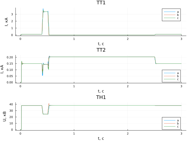
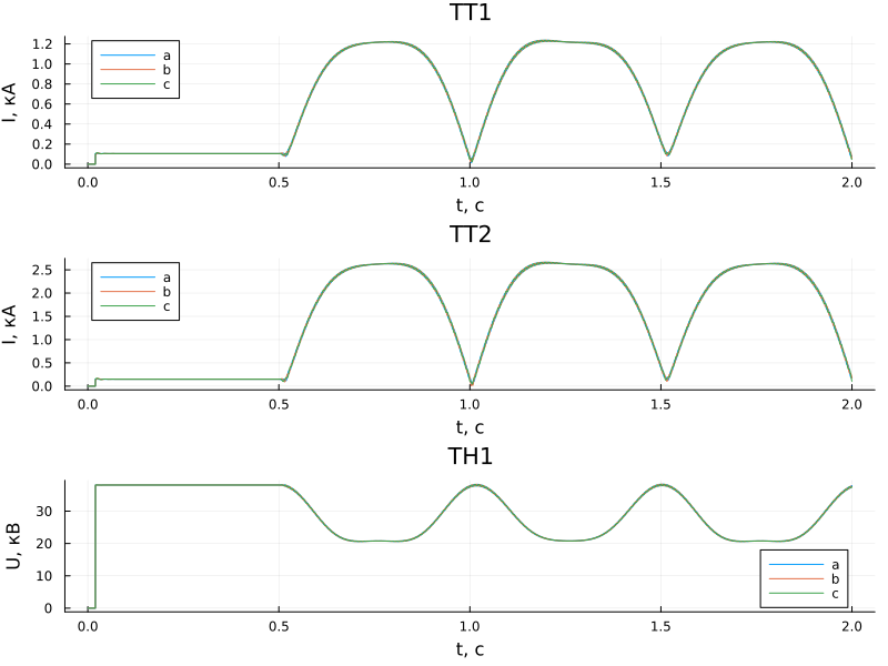
Experiments 21-24
Swing with a swing center on the VL13 line
Test conditions:
- Swing center: on the VL13 line.
- Swing frequency: 1 Hz and increase to failure of the swing lock.
.png)
The model defines experience No. 21. For other experiments, it is necessary to change the amplitude and frequency parameters of the "Sine function" block from the "Frequency" subsystem. For experiment No. 21, the EMF swing angle is set at 2 ± 180° from the set mode. From 0 to 0.5 seconds, the system operates in steady state, and from 0.5 seconds, the frequency begins to change. The amplitude should be increased in proportion to the swing frequency.
model_name = "B3_21_24"
model_name in [m.name for m in engee.get_all_models()] ? engee.open(model_name) : engee.load( "$(@__DIR__)/$(model_name).engee");
results = Vector{Any}(undef, 3)
result = engee.run(model_name);
results[1] = stack(collect(result["I1"].value[:])[!,:value])';
results[2] = stack(collect(result["I2"].value[:])[!,:value])';
results[3] = stack(collect(result["V1"].value[:])[!,:value])';
sim_time = collect(result["I1"].time[:])[!,:time];
Displaying results:
gr()
p1 = plot(sim_time, results[1], title = "TT1",xlabel = "t, with", ylabel = "I, kA", label = ["a" "b" "c"])
p2 = plot(sim_time, results[2], title = "TT2",xlabel = "t, with", ylabel = "I, kA", label = ["a" "b" "c"])
p3 = plot(sim_time, results[3], title = "Line voltage, RMS (PS1)", xlabel = "t, with", ylabel = "U, kV", label = ["ab" "bc" "ca"])
plot(p1, p2, p3, layout=(3,1), size = (800, 600))
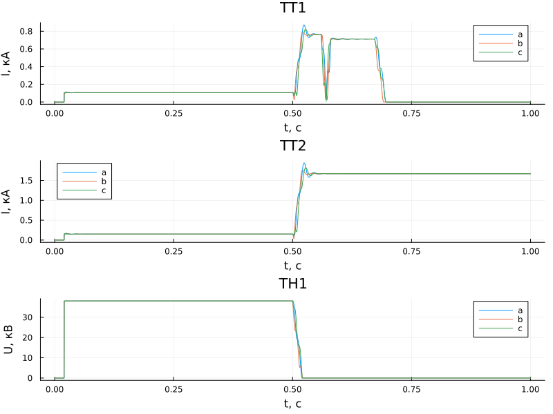
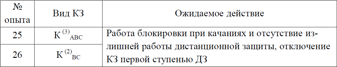
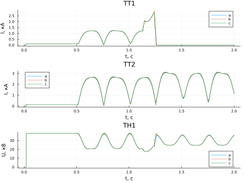
Experience 25-26
Swings with a swing center on the overhead line and short circuit in the area of operation.
Test conditions:
- Swing center: on the VL13 line at a distance of 60% of the line length from the PS3 substation.
- Swing frequency: 2 Hz
- Short circuit location: on the VL13 line at a distance of 40% of the line length from the PS3 substation.
- Type of short circuit: K (3)ABC, K (2)SUN.
.png)
The model has experience number 25. To conduct experiment No. 26, it is necessary to change the type of short circuit in the short circuit block. For experiment No. 25, the EMF swing angle is set at 2 ± 180° from the set mode. From 0 to 0.5 seconds, the system operates in steady state, from 0.5 seconds the frequency begins to change, at 1.125 seconds a short circuit occurs at point K6.
model_name = "B3_25_26"
model_name in [m.name for m in engee.get_all_models()] ? engee.open(model_name) : engee.load( "$(@__DIR__)/$(model_name).engee");
results = Vector{Any}(undef, 3)
result = engee.run(model_name);
results[1] = stack(collect(result["I1"].value[:])[!,:value])';
results[2] = stack(collect(result["I2"].value[:])[!,:value])';
results[3] = stack(collect(result["V1"].value[:])[!,:value])';
sim_time = collect(result["I1"].time[:])[!,:time];
Displaying results:
gr()
p1 = plot(sim_time, results[1], title = "TT1",xlabel = "t, with", ylabel = "I, kA", label = ["a" "b" "c"])
p2 = plot(sim_time, results[2], title = "TT2",xlabel = "t, with", ylabel = "I, kA", label = ["a" "b" "c"])
p3 = plot(sim_time, results[3], title = "Line voltage, RMS (PS1)", xlabel = "t, with", ylabel = "U, kV", label = ["ab" "bc" "ca"])
plot(p1, p2, p3, layout=(3,1), size = (800, 600))
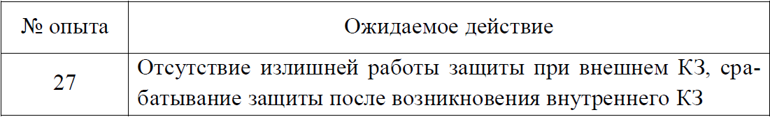
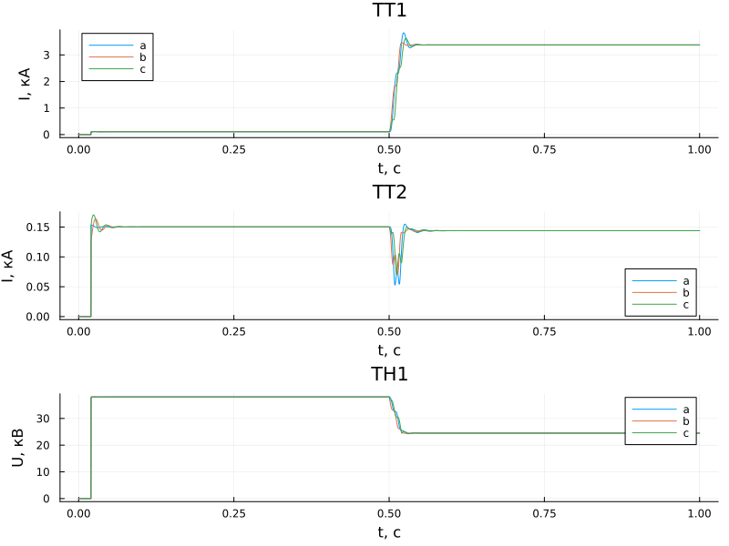
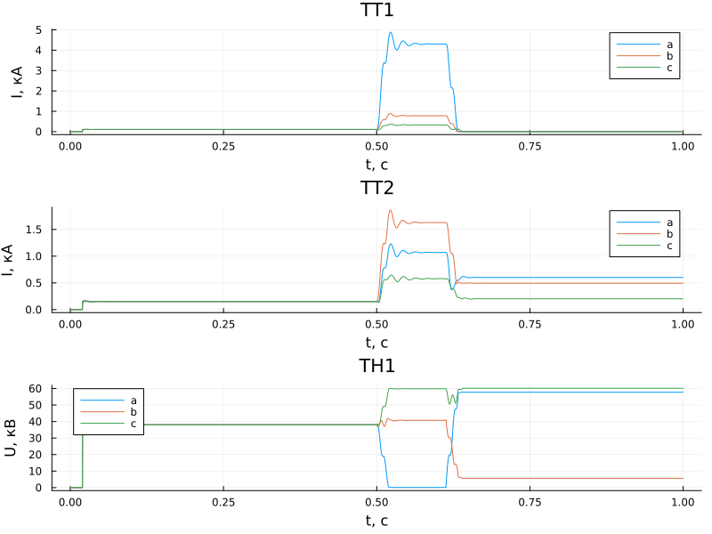
Experience 27
Protection works with an external short circuit that turns into an internal one.
Test conditions:
- Type of short circuit: K (3)
- Short circuit location: PS1 tires (point K4), internal on overhead line 13 (point K3).
- Line load: normal mode.
The sequence of modes:
- Short circuit of the ABC phases on PS1 tires (0.5 s).
- After 60 ms, the short circuit switches to the protected VL13 line (from point K4 to point K3)
.png)
model_name = "B3_27"
model_name in [m.name for m in engee.get_all_models()] ? engee.open(model_name) : engee.load( "$(@__DIR__)/$(model_name).engee");
results = Vector{Any}(undef, 3)
result = engee.run(model_name);
results[1] = stack(collect(result["I1"].value[:])[!,:value])';
results[2] = stack(collect(result["I2"].value[:])[!,:value])';
results[3] = stack(collect(result["V1"].value[:])[!,:value])';
sim_time = collect(result["I1"].time[:])[!,:time];
Displaying results:
gr()
p1 = plot(sim_time, results[1], title = "TT1",xlabel = "t, with", ylabel = "I, kA", label = ["a" "b" "c"])
p2 = plot(sim_time, results[2], title = "TT2",xlabel = "t, with", ylabel = "I, kA", label = ["a" "b" "c"])
p3 = plot(sim_time, results[3], title = "Line voltage, RMS (PS1)", xlabel = "t, with", ylabel = "U, kV", label = ["ab" "bc" "ca"])
plot(p1, p2, p3, layout=(3,1), size = (800, 600))