B1 The program of functional tests of DZ and TNZNP 110-220 kV
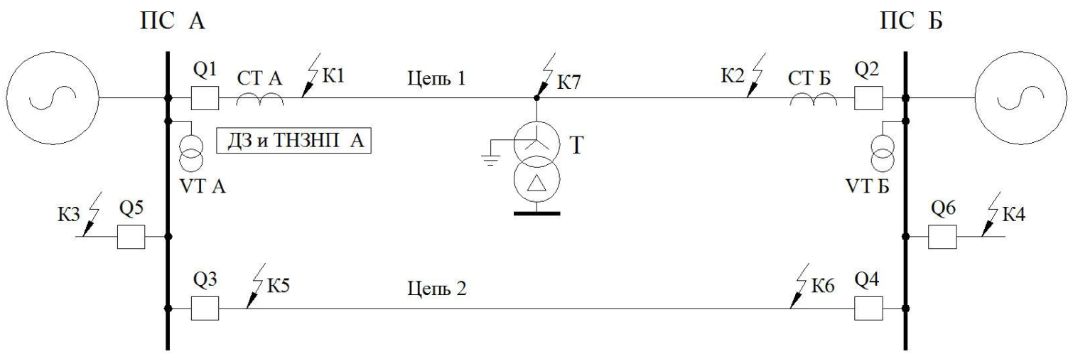
In this example, a test network model is implemented for performing functional tests of DZ and TNZ 110-220 kV from appendix B1 STO 56947007-29.120.70.241-2017. Technical requirements for RPA microprocessor devices. This example contains 12 models named B1_X.engee, where X is the number or range of experiment numbers, the model B1.engee is intended for verification. The model has been adapted and tested for launch at KPM RHYTHM. For more information about using KPM RHYTHM, see the examples KPM RHYTHM: Quick Start and KPM RHYTHM: Real-time operation. Examples of experiments are made to demonstrate without connecting real equipment, you need to connect it yourself. To connect the RPA terminal, you need to add DAC blocks and digital inputs/outputs from the RHYTHM block library to the model, then connect the terminal to the RHYTHM KPM. The scheme of the simulated network:
Parameters of the power system A:
The active resistance of the direct sequence is 4.85 ohms
The inductive resistance of the direct sequence is 25.604 ohms
The active resistance of the zero sequence is 10.607 ohms
The inductive resistance of the zero sequence is 53.347 ohms.
Equivalent EMF– 239 kV
The EMF phase angle is 0°
Power system parameters B:
The active resistance of the direct sequence is 0.393 ohms
The inductive resistance of the direct sequence is 4,276 ohms.
The active resistance of the zero sequence is 0.494 ohms
The inductive resistance of the zero sequence is 4.02 ohms
The equivalent EMF is 239.24 kV
The EMF phase angle is 10.5°
Parameters of the A-B line:
Length 70 km
The resistivity of a straight line is 0.0788 + j 0.4155 ohms/km
The resistivity of the zero-sequence line is 0.3356 + j 1.151 ohms/km
The specific capacity of the direct sequence is 8,594 nF/km
The specific capacity of the zero sequence is 7,305 nF/km
Mutual induction resistivity 0.15 +j 0.684 ohms/km
Transformer on desoldering:
TRDN-40000/220
Snom = 40 MVA
UVH = 230
UHN = 11
Uk = 12 %
Ix = 0.9 %
DRc = 170 kW
DRx = 50 kW
Measuring current transformers:
TFND-220-II
pt= 1200/1 A
Snom = 30 VA, cos φ = 0.8
K10 = 30
Qact = 21.5 cm2
LCP = 106 cm
W1 = 1
W2 = 1200
R2 = 7 ohms
X2 = 0.54 ohms
Model verification
Before the first launch, you need to install a package for rendering tables.:
using Pkg
!("PrettyTables" in [p.name for p in values(Pkg.dependencies())]) && Pkg.add("PrettyTables");
Comparison of required mode parameters and calculated ones:
model_name = "B1"
model_name in [m.name for m in engee.get_all_models()] ? engee.open(model_name) : engee.load( "$(@__DIR__)/$(model_name).engee");
blocks = ["Q1_ctrl", "Q2_ctrl", "Q3_ctrl", "Q4_ctrl", "ZN_3", "ZN_4"]
switch_states = [0 0 0 0 1 1]
for i = 1:length(blocks)
    engee.set_param!(model_name*"/"*blocks[i], "Value" => switch_states[i]);
end
time_ar = [0, 1]
switch = ones(2,4,2)
# Launching the uploaded model:
results = engee.run(model_name);
# simulation time vector
# sim_time = results["P1_1"].time;
P1_1_ex1 = results["P1_1"].value[end]
Q1_1_ex1 = results["Q1_1"].value[end]
V1_1_ex1 = results["V1_1"].value[end][1]
I1_1_ex1 = results["I1_1"].value[end][1]
P2_1_ex1 = results["P2_1"].value[end]
Q2_1_ex1 = results["Q2_1"].value[end]
V2_1_ex1 = results["V2_1"].value[end][1]
I2_1_ex1 = results["I2_1"].value[end][1]
switch_states = [0 0 1 1 0 0]
for i = 1:length(blocks)
    engee.set_param!(model_name*"/"*blocks[i], "Value" => switch_states[i]);
end
# Launching the uploaded model:
results = engee.run(model_name);
# simulation time vector
# sim_time = results["P1_1"].time;
P1_1_ex2 = results["P1_1"].value[end]
Q1_1_ex2 = results["Q1_1"].value[end]
V1_1_ex2 = results["V1_1"].value[end][1]
I1_1_ex2 = results["I1_1"].value[end][1]
P2_1_ex2 = results["P2_1"].value[end]
Q2_1_ex2 = results["Q2_1"].value[end]
V2_1_ex2 = results["V2_1"].value[end][1]
I2_1_ex2 = results["I2_1"].value[end][1];
Disrespect for results:
using PrettyTables
colomn1 = ["Both circuits are in operation", "Bus voltage, kV", "Line current, kA",
"Active power transfer, MW", "Reactive power flow, MVar", "",
"Circuit 2 is disconnected from both sides and grounded", "Bus voltage, kV", "Line current, kA",
"Active power transfer, MW", "Reactive power flow, MVar"]
colomn2 = ["", "239,5", "0,279", "-115", "12,86", "", "", "238,9", "0,420", "-171,7", "25,91"]
colomn3 = ["", "239,8", "0,288", "116,3", "-27,63", "", "", "239,4", "0,428", "174,7", "-31,89"]
colomn4 = ["", V1_1_ex1, I1_1_ex1, P1_1_ex1, Q1_1_ex1, "", "", V1_1_ex2, I1_1_ex2, P1_1_ex2, Q1_1_ex2]
colomn5 = ["", V2_1_ex1, I2_1_ex1, P2_1_ex1, Q2_1_ex1, "", "", V2_1_ex2, I2_1_ex2, P2_1_ex2, Q2_1_ex2]
colomn6 = ["", (239.5 - V1_1_ex1) / 239.5 * 100, (0.279 - I1_1_ex1) / 0.279 * 100, (-115 - P1_1_ex1) / -115 * 100,
(12.86 - Q1_1_ex1) / 12.86 * 100, "", "", (238.9 - V1_1_ex2) / 238.9 * 100, (0.42 - I1_1_ex2) / 0.42 * 100,
(-171.7 - P1_1_ex2) / -171.7 * 100, (25.91 - Q1_1_ex2) / 25.91 * 100]
colomn7 = ["", (239.8 - V2_1_ex1) / 239.8 * 100, (0.288 - I2_1_ex1) / 0.288 * 100, (116.3 - P2_1_ex1) / 116.3 / 100,
(-27.63 - Q2_1_ex1) / -27.63 * 100, "", "", (239.4 - V2_1_ex2) / 239.4 * 100, (0.428 - I2_1_ex2) / 0.428 * 100,
(174.7 - P2_1_ex2) / 174.7 * 100, (-31.89 - Q2_1_ex2) / -31.89 * 100]
data = hcat(colomn1, colomn2, colomn3, colomn4, colomn5, colomn6, colomn7);
header = (["Modes", "PS A", "PS B", "PS A", "PS B", "PS A", "PS B"],
["", "RTDS", "RTDS", "Engee", "Engee", "Mistake, %", "Mistake, %"])
pretty_table(
    data;
    header = header,
    alignment = :l,
    formatters = ft_printf("%5.2f")
)
The calculation error is less than 5%.
Comparison of required short-circuit currents and calculated ones:
switch = []
time_ar = [0, 1]
fault = reshape([0 0 0 1; 0 0 0 1; 1 0 0 0; 1 0 0 0; 0 1 1 0; 0 1 1 0], (6, 4, 1))
fault = cat(fault, fault, dims = 3)
blocks = ["ZN_3", "ZN_4", "Q1_ctrl", "Q2_ctrl","Q3_ctrl","Q4_ctrl","Q5_ctrl","Q6_ctrl"]
switch_states = [1 1 0 0 0 0 1 1; 0 0 0 0 1 1 1 1]
results = Matrix{Any}(undef, 12, 2)
for j = 1:2
    for i = 1:6
        engee.set_param!(model_name*"/"*blocks[i], "Value" => switch_states[j, i]);
    end
    for i = 1:6
        if i % 2 == 1
            switch = cat(reshape(fault[i,:,:], (1,4,2)), ones(5,4,2), dims = 1)
        else
            switch = cat(ones(1,4,2), reshape(fault[i,:,:], (1,4,2)), ones(4,4,2), dims = 1)
        end
        result = engee.run(model_name);
        if i <= 2
            results[i + (j - 1) * 6, 1] = result["I1_1"].value[end][1];
            results[i + (j - 1) * 6, 2] = result["I2_1"].value[end][1];
        else
            results[i + (j - 1) * 6, 1] = result["3I_0_1"].value[end];
            results[i + (j - 1) * 6, 2] = result["3I_0_2"].value[end];
        end
    end
end
Displaying results:
using PrettyTables
I_ref =[8.88 1.7 4.465 0.593 6.13 0.595 5.29 2.47 3.024 1.254 3.744 1.246;
3.61 33.76 1.254 34.67 1.723 34.78 4.06 32.09 2.761 33.79 3.418 33.57]'
colomn1 = ["Both circuits are in operation", "K1", "K2", "K1", "K2","K1", "K2",
"Circuit 2 is disconnected from both sides and grounded", "K1", "K2","K1", "K2", "K1", "K2"]
colomn2 = ["", "K(3)", "K(3)", "K(1,1)", "K(1,1)", "K(1)", "K(1)", "","K(3)", "K(3)", "K(1,1)", "K(1,1)", "K(1)", "K(1)"]
colomn3 = ["", "I1", "I1", "3I0", "3I0", "3I0", "3I0", "", "I1", "I1", "3I0", "3I0", "3I0", "3I0"]
colomn4 = ["", "8.88", "1.7", "4.465", "0.593", "6.13", "0.595", "", "5.29", "2.47", "3.024", "1.254", "3.744", "1.246"]
colomn5 = ["", "3.61", "33.76", "1.254", "34.67", "1.723", "34.78", "", "4.06", "32.09", "2.761", "33.79", "3.418", "33.57"]
colomn6 = reshape(cat("", transpose(results[1:6,1]),"", transpose(results[7:12,1]), dims=2), (14))
colomn7 = reshape(cat("", transpose(results[1:6,2]),"", transpose(results[7:12,2]), dims=2), (14))
colomn8 = reshape(cat("", (results[1:6,1]-I_ref[1:6,1])./I_ref[1:6,1].*100,
"", (results[7:12,1]-I_ref[7:12,1])./I_ref[7:12,1].*100, dims=1), (14))
colomn9 = reshape(cat("", (results[1:6,2]-I_ref[1:6,2])./I_ref[1:6,2].*100,
"", (results[7:12,2]-I_ref[7:12,2])./I_ref[7:12,2].*100, dims=1), (14))
data = hcat(colomn1, colomn2, colomn3, colomn4, colomn5, colomn6, colomn7, colomn8, colomn9);
header = (["Short circuit modes", "", "", "from PS A", "from PS B", "from PS A", "from PS B", "from PS A", "from PS B"],
["KZ location", "Type of short circuit", "", "RTDS", "RTDS", "Engee", "Engee", "Mistake, %", "Mistake, %"])
pretty_table(
    data;
    header = header,
    alignment = :l,
    formatters = ft_printf("%5.2f")
)
The calculation error is less than 5%.
Experiments 1-10
The effect of transient resistance and load on the operation of the remote control with internal short circuits.
Test conditions:
- KZ location: point K4.
- Type of short circuit: K(1,1)VS0, K(1)B0
Experiment parameters:
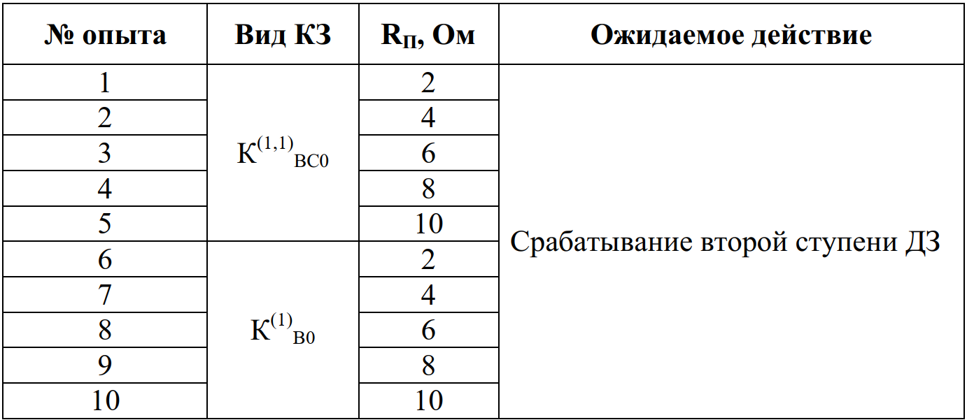
Experiment No. 1 is set in the model. To conduct other experiments, it is necessary to change the type of short circuit and the transient resistance in the short circuit block.
model_name = "B1_1_10"
model_name in [m.name for m in engee.get_all_models()] ? engee.open(model_name) : engee.load( "$(@__DIR__)/$(model_name).engee");
results = Matrix{Any}(undef, 1, 4)
result = engee.run(model_name);
results[1, 1] = stack(collect(result["I1_1"].value[:])[!,:value])';
results[1, 2] = stack(collect(result["I2_1"].value[:])[!,:value])';
results[1, 3] = stack(collect(result["V1_1"].value[:])[!,:value])';
results[1, 4] = stack(collect(result["V2_1"].value[:])[!,:value])';
sim_time = collect(result["I1_1"].time[:])[!,:time];
Displaying results:
# measuring side, 1 - PS A, 2 -PS B
dir = 1;
gr()
p1 = plot(sim_time, results[1, dir], title = "Primary current, RMS", xlabel = "t, with", ylabel = "I, kA", label = ["a" "b" "c"])
p2 = plot(sim_time, results[1, dir + 2], title = "Line voltage, RMS", xlabel = "t, with", ylabel = "U, kV", label = ["a" "b" "c"])
plot(p1, p2, layout=(2,1), )
Experiments 11-14
Checking the operation of the remote control with close short circuits.
Test conditions:
- Type of short circuit: K(3)ABC
- Transient resistance at the short circuit location: 0 Ohms.
Experiment parameters:
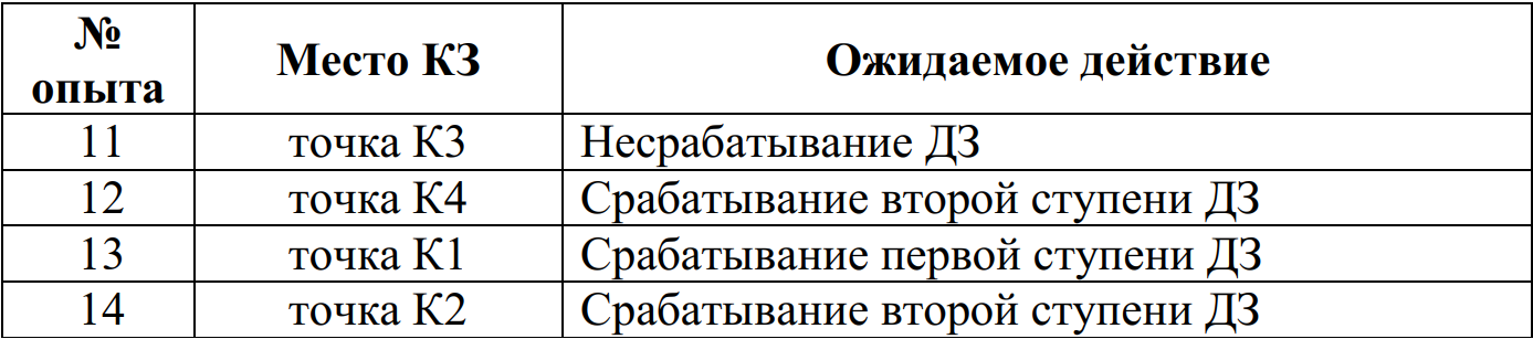
The model defines experience No. 11. For other experiments, it is necessary to move the short circuit unit to the required point.
model_name = "B1_11_14"
model_name in [m.name for m in engee.get_all_models()] ? engee.open(model_name) : engee.load( "$(@__DIR__)/$(model_name).engee");
results = Matrix{Any}(undef, 1, 4)
result = engee.run(model_name);
results[1, 1] = stack(collect(result["I1_1"].value[:])[!,:value])';
results[1, 2] = stack(collect(result["I2_1"].value[:])[!,:value])';
results[1, 3] = stack(collect(result["V1_1"].value[:])[!,:value])';
results[1, 4] = stack(collect(result["V2_1"].value[:])[!,:value])';
sim_time = result["I1_1"].time;
Displaying results:
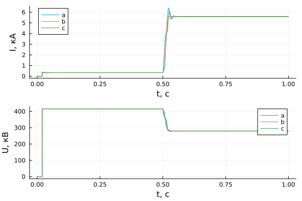
# measuring side, 1 - PS A, 2 -PS B
dir = 1;
gr()
p1 = plot(sim_time, results[1, dir], title = "Primary current, RMS", xlabel = "t, with", ylabel = "I, kA", label = ["a" "b" "c"])
p2 = plot(sim_time, results[1, dir + 2], title = "Line voltage, RMS", xlabel = "t, with", ylabel = "U, kV", label = ["a" "b" "c"])
plot(p1, p2, layout=(2,1))
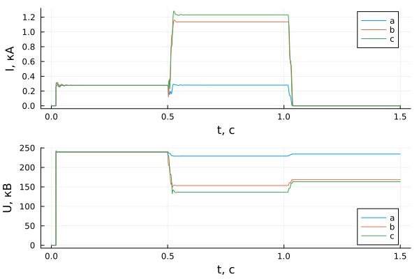
Experience 15-16
Checking the operation of the fuel pump with external short circuits on the tires
Test conditions:
- KZ location: point K3, point K4.
- Type of short circuit: K(1)A0.
- Transient resistance at the short circuit location: 0 Ohms.
- The parallel line is disconnected from both sides and grounded.
- Normal load mode, preceding short circuit.
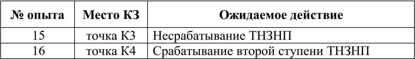
The model has experience number 15. To carry out experiment No. 16, it is necessary to move the short circuit block to the required point.
model_name = "B1_15_16"
model_name in [m.name for m in engee.get_all_models()] ? engee.open(model_name) : engee.load( "$(@__DIR__)/$(model_name).engee");
results = Matrix{Any}(undef, 1, 4)
result = engee.run(model_name);
results[1, 1] = stack(collect(result["I1_1"].value[:])[!,:value])';
results[1, 2] = stack(collect(result["I2_1"].value[:])[!,:value])';
results[1, 3] = stack(collect(result["V1_1"].value[:])[!,:value])';
results[1, 4] = stack(collect(result["V2_1"].value[:])[!,:value])';
sim_time = result["I1_1"].time;
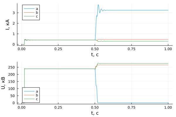
Displaying results:
# measuring side, 1 - PS A, 2 -PS B
dir = 1;
gr()
p1 = plot(sim_time, results[1, dir], title = "Primary current, RMS", xlabel = "t, with", ylabel = "I, kA", label = ["a" "b" "c"])
p2 = plot(sim_time, results[1, dir + 2], title = "Line voltage, RMS", xlabel = "t, with", ylabel = "U, kV", label = ["a" "b" "c"])
plot(p1, p2, layout=(2,1))
Experience 17-20
Checking the operation of the DZ and TNNP with an internal short circuit with a successful TAP.
The sequence of modes:
- 0-0.4 s Normal load mode, preceding short circuit
- 0.4 s Occurrence of short circuit in the middle of the overhead line.
- 0.5 s Three-phase disconnection of the line with protections on both sides.
- 1 with the disappearance of the KZ. Shockless pause (1.5 s)
- 2 s TAP from the side of the control panel due to the absence of voltage
- 2.5 s "Blind" TAPV on the side of PS B.
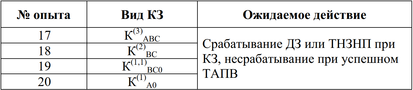
The model defines experience No. 17. For other experiments, it is necessary to change the type of short circuit in the short circuit block.
model_name = "B1_17_20"
model_name in [m.name for m in engee.get_all_models()] ? engee.open(model_name) : engee.load( "$(@__DIR__)/$(model_name).engee");
results = Matrix{Any}(undef, 1, 4)
result = engee.run(model_name);
results[1, 1] = stack(collect(result["I1_1"].value[:])[!,:value])';
results[1, 2] = stack(collect(result["I2_1"].value[:])[!,:value])';
results[1, 3] = stack(collect(result["V1_1"].value[:])[!,:value])';
results[1, 4] = stack(collect(result["V2_1"].value[:])[!,:value])';
sim_time = collect(result["I1_1"].time[:])[!,:time];
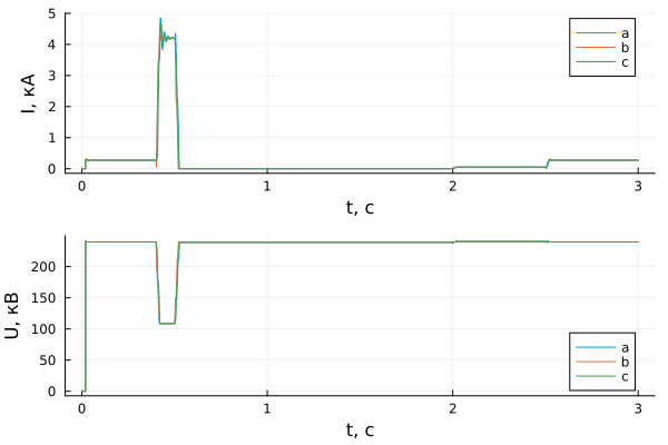
Displaying results:
# measuring side, 1 - PS A, 2 -PS B
dir = 1;
gr()
p1 = plot(sim_time, results[1, dir], title = "Primary current, RMS", xlabel = "t, with", ylabel = "I, kA", label = ["a" "b" "c"])
p2 = plot(sim_time, results[1, dir+2], title = "Line voltage, RMS", xlabel = "t, with", ylabel = "U, kV", label = ["a" "b" "c"])
plot(p1, p2, layout=(2,1))
Experiments 21-24
Checking the operation of the DZ and TNNP with an internal short circuit with an unsuccessful TAP.
The sequence of modes:
- 0-0.4 s Normal load mode, preceding short circuit.
- 0.4 s Short circuit occurrence.
- 0.5 s Three-phase disconnection of the line with protections on both sides.
- 2 s TAP from the side of PS A (1.5 s).
- 2.1 s Disconnection of the line from the protection of PS A.
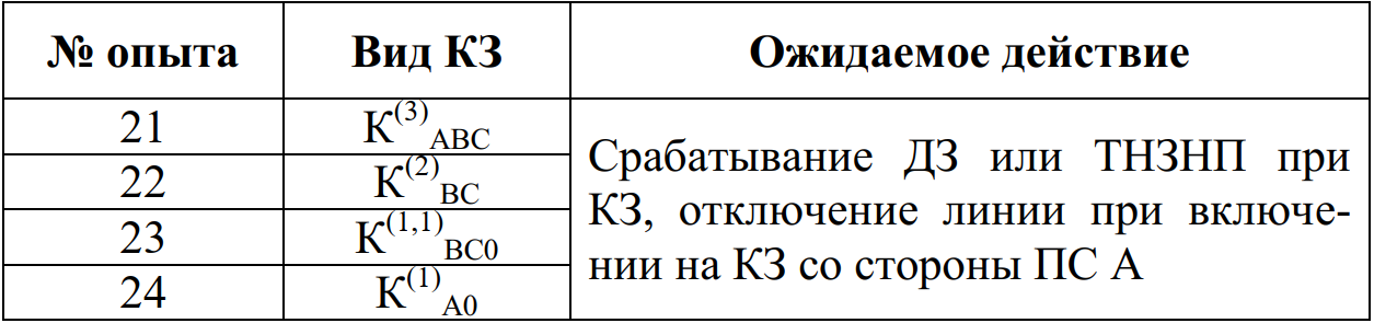
The model defines experience No. 21. For other experiments, it is necessary to change the type of short circuit in the short circuit block.
model_name = "B1_21_24"
model_name in [m.name for m in engee.get_all_models()] ? engee.open(model_name) : engee.load( "$(@__DIR__)/$(model_name).engee");
results = Matrix{Any}(undef, 1, 4)
result = engee.run(model_name);
results[1, 1] = stack(collect(result["I1_1"].value[:])[!,:value])';
results[1, 2] = stack(collect(result["I2_1"].value[:])[!,:value])';
results[1, 3] = stack(collect(result["V1_1"].value[:])[!,:value])';
results[1, 4] = stack(collect(result["V2_1"].value[:])[!,:value])';
sim_time = collect(result["I1_1"].time[:])[!,:time];
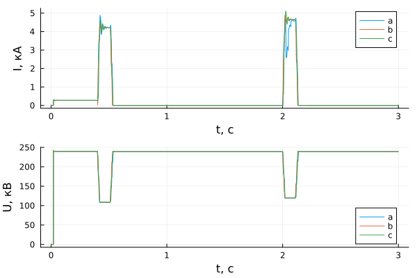
Displaying results:
# measuring side, 1 - PS A, 2 -PS B
dir = 1
gr()
p1 = plot(sim_time, results[1, dir], title = "Primary current, RMS", xlabel = "t, with", ylabel = "I, kA", label = ["a" "b" "c"])
p2 = plot(sim_time, results[1, dir+2], title = "Line voltage, RMS", xlabel = "t, with", ylabel = "U, kV", label = ["a" "b" "c"])
plot(p1, p2, layout=(2,1))
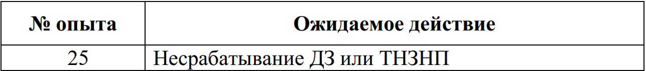
Experience 25
Checking the operation of the DZ and TNNP with external short circuits with unsuccessful TAPV with TT saturation.
The sequence of modes:
- 0-0.4 s Normal load mode.
- 0.4 s Short circuit occurrence.
- 0.5 s After 100 ms disconnection of the damaged line.
- 1.5 s APV from the side of PS A (1 s).
- 1.6 s After 100 ms disconnection of the damaged line.
model_name = "B1_25"
model_name in [m.name for m in engee.get_all_models()] ? engee.open(model_name) : engee.load( "$(@__DIR__)/$(model_name).engee");
results = Matrix{Any}(undef, 1, 4)
result = engee.run(model_name);
results[1, 1] = stack(collect(result["I1_1"].value[:])[!,:value])';
results[1, 2] = stack(collect(result["I2_1"].value[:])[!,:value])';
results[1, 3] = stack(collect(result["V1_1"].value[:])[!,:value])';
results[1, 4] = stack(collect(result["V2_1"].value[:])[!,:value])';
sim_time =  collect(result["I1_1"].time[:])[!,:time];
Displaying results:
# measuring side, 1 - PS A, 2 -PS B
dir = 2
gr()
p1 = plot(sim_time, results[1, dir], title = "Primary current, RMS", xlabel = "t, with", ylabel = "I, kA", label = ["a" "b" "c"])
p2 = plot(sim_time, results[1, dir+2], title = "Line voltage, RMS", xlabel = "t, with", ylabel = "U, kV", label = ["a" "b" "c"])
plot(p1, p2, layout=(2,1))
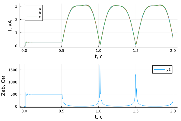
Experiments 26-29
Swing with the swing center on the A-B line.
Test conditions:
- Swing center: measuring the resistance at PS A falls into the first zone of the DZ.
- Swing frequency: 1 Hz and increase to failure of the swing lock.
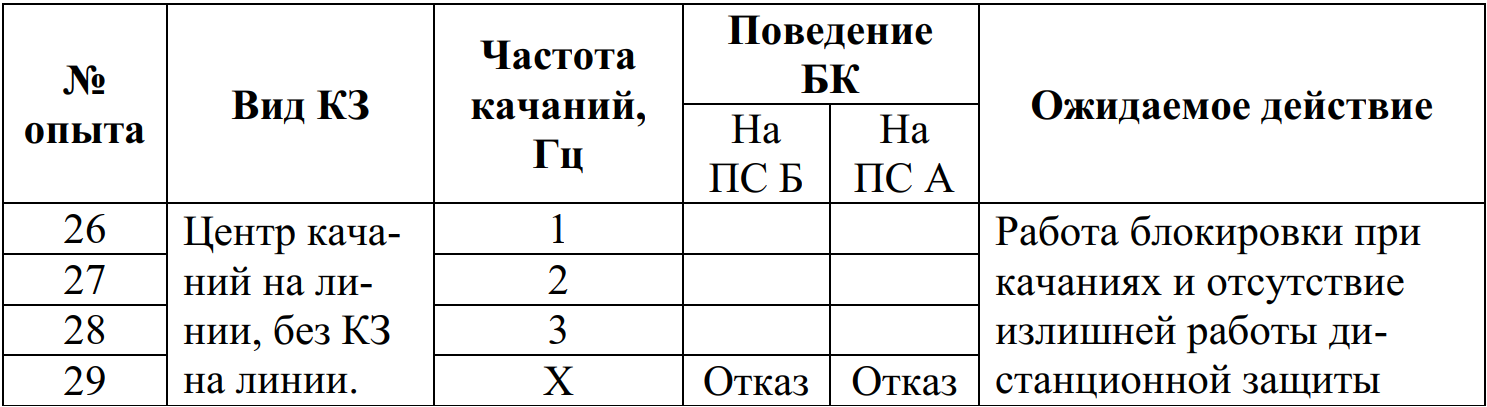
Experiment No. 26 is set in the model. To conduct other experiments, it is necessary to change the amplitude and frequency parameters of the "Sinusoidal function" block from the "Frequency" subsystem. For experiment No. 26, the EMF swing angle at PS B is set to ± 180° from the set mode. From 0 to 0.5 seconds, the system operates in steady state, and from 0.5 seconds, the frequency begins to change. The amplitude should be increased in proportion to the swing frequency.
model_name = "B1_26_29"
model_name in [m.name for m in engee.get_all_models()] ? engee.open(model_name) : engee.load( "$(@__DIR__)/$(model_name).engee");
results = Matrix{Any}(undef, 1, 4)
result = engee.run(model_name);
results[1, 1] = stack(collect(result["I1_1"].value[:])[!,:value])';
results[1, 2] = stack(collect(result["I2_1"].value[:])[!,:value])';
results[1, 3] = stack(collect(result["Zab_1"].value[:])[!,:value]);
results[1, 4] = stack(collect(result["Zab_2"].value[:])[!,:value]);
sim_time =  collect(result["I1_1"].time[:])[!,:time];
Displaying results:
# measuring side, 1 - PS A, 2 -PS B
dir = 1
gr()
p1 = plot(sim_time, results[1, dir], title = "Primary current, RMS", xlabel = "t, with", ylabel = "I, kA", label = ["a" "b" "c"])
p2 = plot(sim_time, results[1, dir+2], title = "Resistance", xlabel = "t, with", ylabel = "Zab, Om")
plot(p1, p2, layout=(2,1))
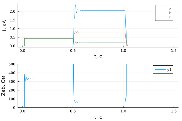
Experiments 30-37
Swing with the swing center on the A-B line and short circuit in the protection area.
Test conditions:
- Swing center: measuring the resistance at PS A falls into the first zone of the DZ.
- Swing frequency: 2 Hz.
- KZ location: 40% of PS B.
- Type of short circuit: K(3)ABC, K(2)BC, K(1,1)BC0, K(1)A0
- The resistance at the short-circuit point is 0 and 10 ohms.
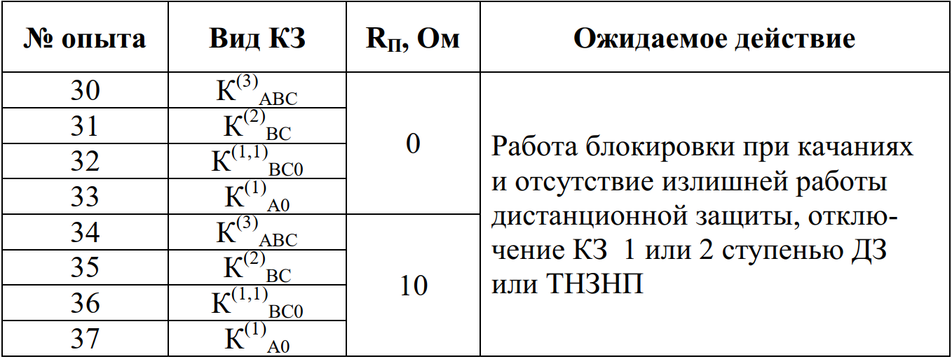
The model has experience number 30. For other experiments, it is necessary to change the type of short circuit and the transient resistance in the short circuit block. For experiment No. 30, the EMF swing angle at PS B is set to ± 180° from the set mode. From 0 to 0.5 seconds, the system operates in steady state, from 0.5 seconds the frequency begins to change, at 1.125 seconds a short circuit occurs at point K7.
model_name = "B1_30_37"
model_name in [m.name for m in engee.get_all_models()] ? engee.open(model_name) : engee.load( "$(@__DIR__)/$(model_name).engee");
results = Matrix{Any}(undef, 1, 4)
result = engee.run(model_name);
results[1, 1] = stack(collect(result["I1_1"].value[:])[!,:value])';
results[1, 2] = stack(collect(result["I2_1"].value[:])[!,:value])';
results[1, 3] = stack(collect(result["Zab_1"].value[:])[!,:value]);
results[1, 4] = stack(collect(result["Zab_2"].value[:])[!,:value]);
sim_time =  collect(result["I1_1"].time[:])[!,:time];
Displaying results:
# Experience number
n = 1;
# measuring side, 1 - PS A, 2 -PS B
dir = 1
gr()
p1 = plot(sim_time, results[n, dir], title = "Primary current, RMS", xlabel = "t, with", ylabel = "I, kA", label = ["a" "b" "c"])
p2 = plot(sim_time, results[n, dir+2], title = "Resistance", xlabel = "t, with", ylabel = "Zab, Om", ylims = (0, 1500))
plot(p1, p2, layout=(2,1))
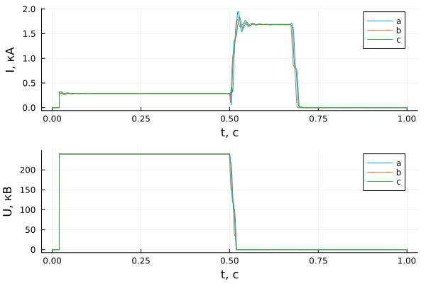
Experience 38
Checking the operation of the remote control with an external short circuit on a parallel line passing into an internal one.
Test conditions:
- Type of short circuit: External to (3)ABC, turning into internal.
- Location of the KZ: at PS B on an adjacent parallel line, inside at PS B.
- Line load: normal mode.
- The angle of occurrence of short circuit: 0°.
- The transient resistance at the short-circuit point is 0 ohms.
The sequence of modes is:
- 0.4995 s short circuit ABC on the parallel line from the side of PS B (point K4).
- 0.5995 s short circuit switches to the protected line (point K2).
model_name = "B1_38"
model_name in [m.name for m in engee.get_all_models()] ? engee.open(model_name) : engee.load( "$(@__DIR__)/$(model_name).engee");
results = Matrix{Any}(undef, 1, 4)
result = engee.run(model_name);
results[1, 1] = stack(collect(result["I1_1"].value[:])[!,:value])';
results[1, 2] = stack(collect(result["I2_1"].value[:])[!,:value])';
results[1, 3] = stack(collect(result["V1_1"].value[:])[!,:value])';
results[1, 4] = stack(collect(result["V2_1"].value[:])[!,:value])';
sim_time = collect(result["I1_1"].time[:])[!,:time];
Displaying results:
# measuring side, 1 - PS A, 2 -PS B
dir = 2
gr()
p1 = plot(sim_time, results[1, dir], title = "Primary current, RMS", xlabel = "t, with", ylabel = "I, kA", label = ["a" "b" "c"])
p2 = plot(sim_time, results[1, dir+2], title = "Line voltage, RMS", xlabel = "t, with", ylabel = "U, kV", label = ["a" "b" "c"])
plot(p1, p2, layout=(2,1))
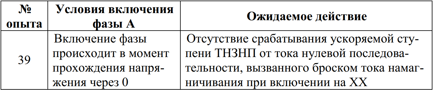
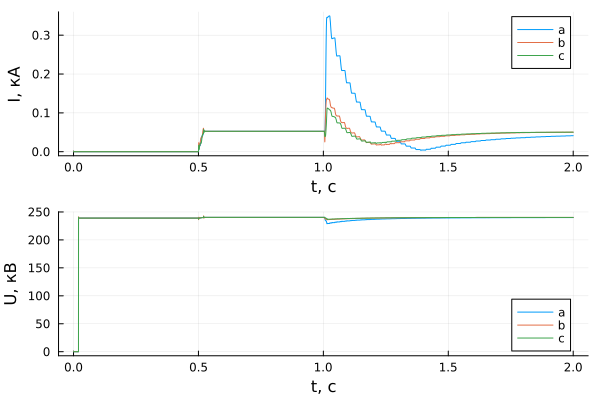
Experience 39
Checking the operation of the fuel pump when the transformer on the overhead line branch is turned on at idle.
Test conditions:
- The line is disconnected from both sides and is not grounded.
- The transformer switch on the branch is off.
The sequence of modes:
- 0 with overhead line disconnected on both sides.
- 0.5 s Switching on the overhead line at idle from the side of PS A.
- 1 s Switching on the transformer at idle.
model_name = "B1_39"
model_name in [m.name for m in engee.get_all_models()] ? engee.open(model_name) : engee.load( "$(@__DIR__)/$(model_name).engee");
results = Matrix{Any}(undef, 1, 4)
result = engee.run(model_name);
results[1, 1] = stack(collect(result["I1_1"].value[:])[!,:value])';
results[1, 2] = stack(collect(result["I2_1"].value[:])[!,:value])';
results[1, 3] = stack(collect(result["V1_1"].value[:])[!,:value])';
results[1, 4] = stack(collect(result["V2_1"].value[:])[!,:value])'
sim_time = collect(result["I1_1"].time[:])[!,:time];
Displaying results:
# measuring side, 1 - PS A, 2 -PS B
dir = 1
gr()
p1 = plot(sim_time, results[1, dir], title = "Primary current, RMS", xlabel = "t, with", ylabel = "I, kA", label = ["a" "b" "c"])
p2 = plot(sim_time, results[1, dir+2], title = "Line voltage, RMS", xlabel = "t, with", ylabel = "U, kV", label = ["a" "b" "c"])
plot(p1, p2, layout=(2,1))
Experiments 40-41
Checking the effect of mutual induction of a parallel line on the operation of a remote control system.
Test conditions:
- Normal mode.
- KZ location: point K4.
- Short circuit type: K(1)A0
- The transient resistance at the short-circuit point is 0 ohms.
- a) The parallel line is disconnected and grounded.
- b) Parallel line in operation.
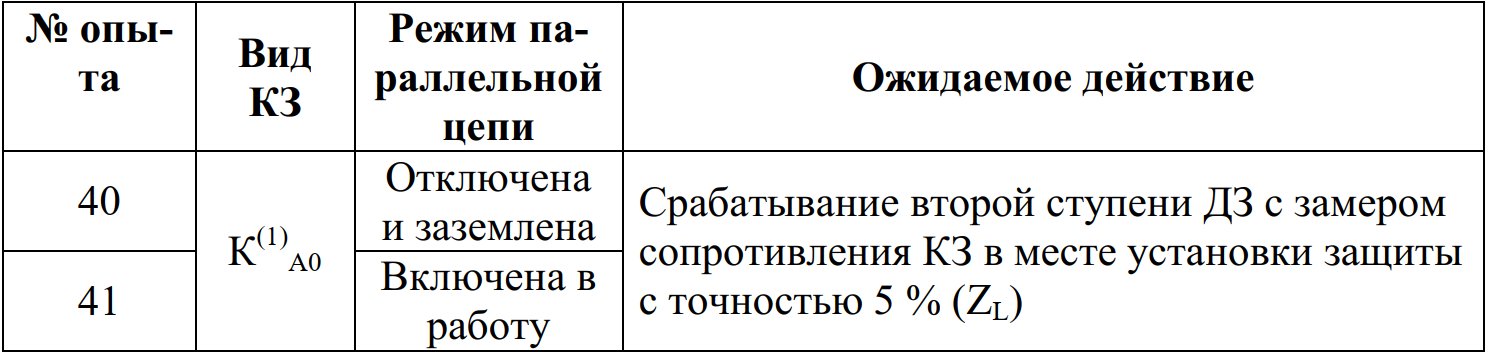
Experience #40 is set in the model. To carry out experiment No. 41, it is necessary to turn on switches Q3 and Q4, turn off the switches of the grounding knives.
model_name = "B1_40_41"
model_name in [m.name for m in engee.get_all_models()] ? engee.open(model_name) : engee.load( "$(@__DIR__)/$(model_name).engee");
results = Matrix{Any}(undef, 1, 4)
result = engee.run(model_name);
results[1, 1] = stack(collect(result["I1_1"].value[:])[!,:value])';
results[1, 2] = stack(collect(result["I2_1"].value[:])[!,:value])';
results[1, 3] = stack(collect(result["Zab_1"].value[:])[!,:value]);
results[1, 4] = stack(collect(result["Zab_2"].value[:])[!,:value]);
sim_time = collect(result["I1_1"].time[:])[!,:time];
Displaying results:
# measuring side, 1 - PS A, 2 -PS B
dir = 1
gr()
p1 = plot(sim_time, results[1, dir], title = "Primary current, RMS", xlabel = "t, with", ylabel = "I, kA", label = ["a" "b" "c"])
p2 = plot(sim_time, results[1, dir+2], title = "Resistance", xlabel = "t, with", ylabel = "Zab, Om", ylims = (0, 500))
plot(p1, p2, layout=(2,1))