Comparison of AC/DC converter modeling techniques

Description of the model

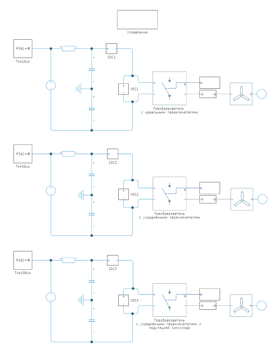
This example shows how to use various modeling techniques for AC/DC converters. The model contains three converters:

Converter with perfect switches — to achieve high detail, this model uses perfect switches and protective diodes, with a sampling period of 10 microseconds.
Converter with averaged switches — to achieve high detail, even with a sampling period of 50 microseconds, this model uses averaged switches with averaged PWM signals.
Converter with averaged switches and sine wave modulation — to maximize the sampling period and work as an ideal averaged converter, this model uses averaged switches and a sine wave signal instead of PWM signals, the sampling period is 100 microseconds.

The level of detail is adjusted by changing the values of the Switch type parameter. Using a more detailed model increases the accuracy of the results, but also slows down the simulation.

Model

Simulation results

Loading the model:

model_name = "power_converter_fidelity";
model_name in [m.name for m in engee.get_all_models()] ? engee.open(model_name) : engee.load("$(@__DIR__)/$(model_name).engee");

Launching the model:

results = engee.run(model_name);

To import the simulation results, logging of the necessary signals was enabled in advance and their names were set. Converting the simulation results from the results variable:

# simulation time vector
sim_time = results["vabc1"].time;
# vectors of recorded signals
va1 = stack(results["vabc1"].value)'[:,1];
va2 = stack(results["vabc2"].value)'[:,1];
va3 = stack(results["vabc3"].value)'[:,1];
va_en = hcat(va1,va2,va3);
ia1 = stack(results["iabc1"].value)'[:,1];
ia2 = stack(results["iabc2"].value)'[:,1];
ia3 = stack(results["iabc3"].value)'[:,1];
ia_en = hcat(ia1,ia2,ia3);
iDC1 = results["iDC1"].value;
iDC2 = results["iDC2"].value;
iDC3 = results["iDC3"].value;
iDC_en = hcat(iDC1,iDC2,iDC3);
va1 = stack(results["vabc1"].value)'[:,1];
va2 = stack(results["vabc2"].value)'[:,1];
va3 = stack(results["vabc3"].value)'[:,1];
va_en = hcat(va1,va2,va3);

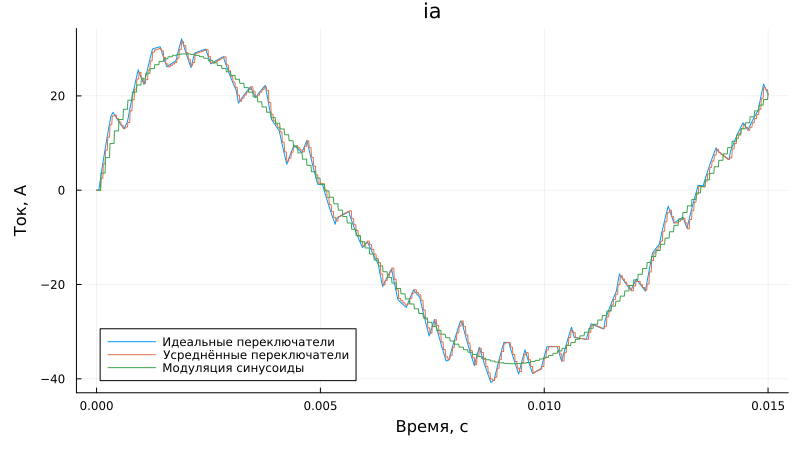
Graph of currents in phase A on the load side:

using Plots;
gr();
plot(sim_time, ia1, label = "Perfect switches", xlabel = "Time, from", left_margin=5Plots.mm)
plot!(sim_time, ia2, label = "Averaged switches", ylabel = "Current, A", bottom_margin=5Plots.mm)
plot!(sim_time, ia3, label = "Sinusoid modulation", title = "ia", size = (800,450))

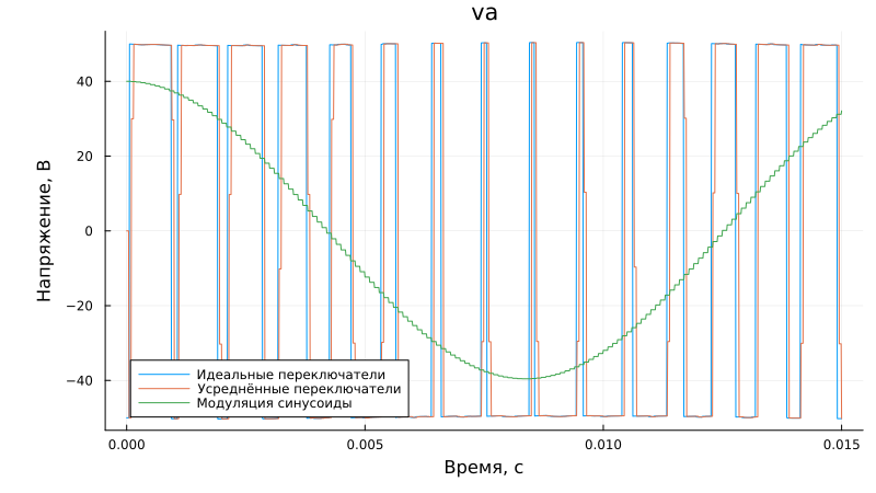
Voltage graph of phase A on the load side:

plot(sim_time, va1, label = "Perfect switches", xlabel = "Time, from", left_margin=10Plots.mm)
plot!(sim_time, va2, label = "Averaged switches", ylabel = "Voltage, V", bottom_margin=5Plots.mm)
plot!(sim_time, va3, label = "Sinusoid modulation", title = "va", size = (800,450))

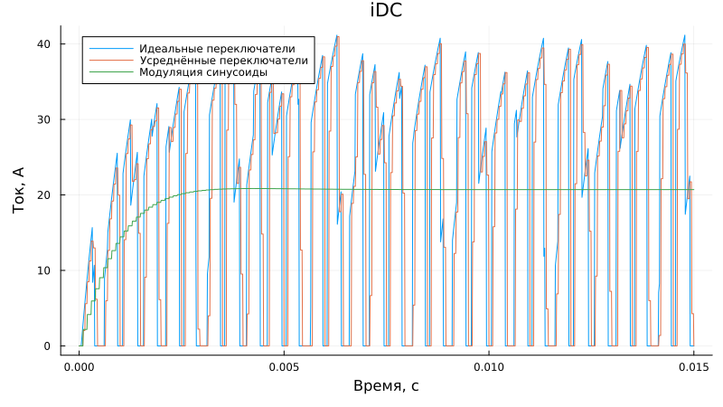
Currents consumed by converters from the direct current side:

gr()
plot(sim_time, iDC1, label = "Perfect switches", xlabel = "Time, from", left_margin=5Plots.mm)
plot!(sim_time, iDC2, label = "Averaged switches", ylabel = "Current, A", bottom_margin=5Plots.mm)
plot!(sim_time, iDC3, label = "Sinusoid modulation", title = "iDC", size = (800,450))

The considered modeling techniques can be applied as follows:

Detailed model — used for the final stage of development or for real-time simulation on [KPM RHYTHM] (https://engee.com/community/ru/catalogs/projects/kpm-ritm-bystryi-start ) using FPGAs.
The averaged PWM averaged model is a compromise between accuracy and simulation speed. It can be used at the development stage of a device and control system, or for real-time simulation on a KPM RHYTHM using a central processor.
An average sinusoid modulated model is the fastest way to model, but also less accurate in terms of transients. It can be used at the stage of development of devices and control systems or for real-time simulation on a KPM RHYTHM using a central processor.

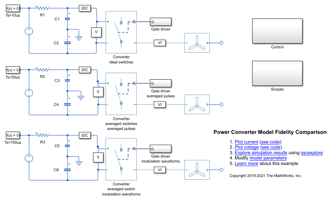
Comparison of simulation results with a similar model in Simulink.

The model is developed by analogy with the example in Simulink Power Converter Model Fidelity Comparison. The model's appearance:

The signals from the Simulink model were pre-recorded and saved to mat files. Downloading data from mat files:

using MAT
data = matread("$(@__DIR__)/iDC.mat")
iDC = data["iDC"]';
data2 = matread("$(@__DIR__)/ia.mat")
ia = data2["ia"]';
data3 = matread("$(@__DIR__)/va.mat")
va = data3["va"]';

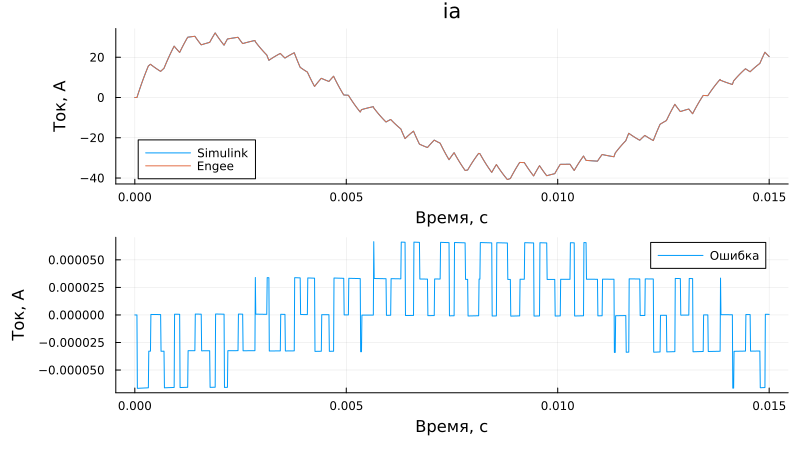
Comparison of currents in phase A on the load side

n = 1; # converter number from top to bottom
p1 = plot(ia[:,1], ia[:,n+1], label = "Simulink", title = "ia")
plot!(p1, sim_time, ia_en[:,n], label = "Engee", left_margin=15Plots.mm)
p2 = plot(ia[:,1], ia_en[:,n] - ia[:,n+1], label = "Mistake", bottom_margin=5Plots.mm)
plot(p1, p2, layout=(2,1), size = (800,450), xlabel = "Time, from", ylabel = "Current, A")

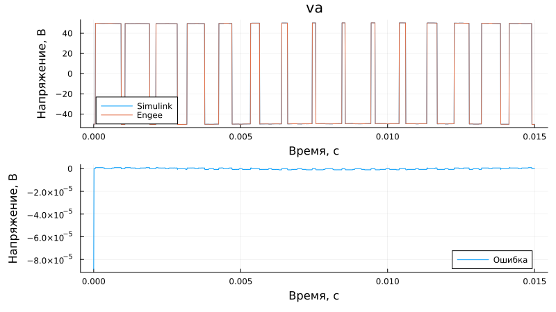
Comparison of phase A voltages on the load side:

n = 1; # converter number from top to bottom
p1 = plot(va[:,1], va[:,n+1], label = "Simulink", title = "va")
plot!(p1, sim_time, va_en[:,n], label = "Engee", left_margin=15Plots.mm)
p2 = plot(va[:,1], va_en[:,n] - va[:,n+1], label = "Mistake", bottom_margin=5Plots.mm)
plot(p1, p2, layout=(2,1), size = (800,450), xlabel = "Time, from", ylabel = "Voltage, V")

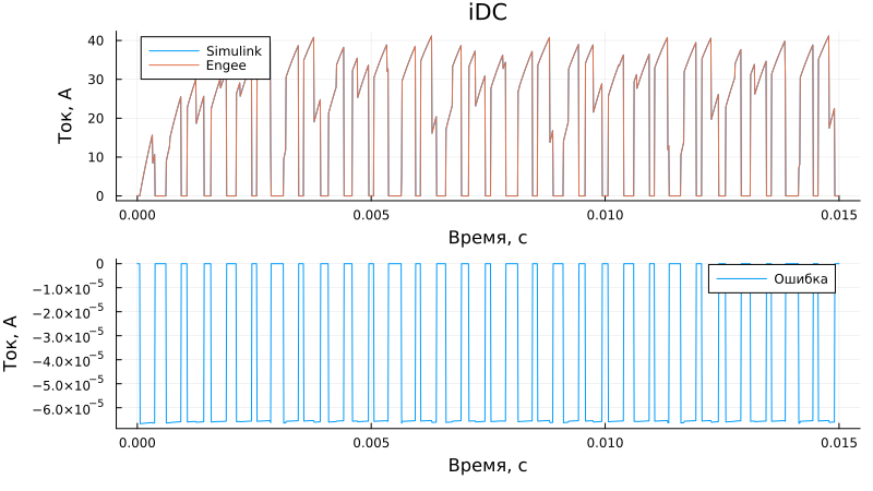
Comparison of currents consumed by converters from the direct current side:

n = 1; # converter number from top to bottom
p1 = plot(iDC[:,1], iDC[:,n+1], label = "Simulink", title = "iDC")
plot!(p1, sim_time, iDC_en[:,n], label = "Engee", left_margin=15Plots.mm)
p2 = plot(iDC[:,1], iDC_en[:,n] - iDC[:,n+1], label = "Mistake", bottom_margin=5Plots.mm)
plot(p1, p2, layout=(2,1), size = (800,450), xlabel = "Time, from", ylabel = "Current, A")