Rapid prototyping of a garland control algorithm

On the eve of the New Year, you always want to create a special atmosphere. This example shows how, using KPM RHYTHM, you can develop an algorithm for controlling an LED garland that will change its brightness depending on the volume of the music, creating the effect of "dancing lights."

This example shows how to use a real—time machine, KPM RHYTHM, for rapid prototyping of control algorithms. The control object is an LED garland. The control algorithm adjusts the brightness of the garland in proportion to the volume of the music. First, the audio file is processed using a script, and then the received signal is loaded into the KPM RHYTHM model.

The model running on KPM RHYTHM contains a subsystem Звуковой сигнал, in which a vector of processed audio file amplitude values is loaded from the workspace. In the first 2 seconds, the subsystem outputs a value of 1 for audio synchronization. The signal is played cyclically — after reaching the end of the audio file, it is played from the beginning.

The amplitude of the signal, which has values from 0 to 1, is multiplied by the voltage gain factor of -5. The coefficient has a negative value because a voltage lower than the anode must be applied to the cathode of the LED.

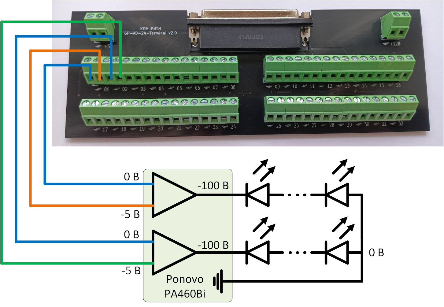
The amplified signal is then applied to the unit GP-AD-24 DAC, which controls the built-in digital-to-analog conversion module (DAC). The maximum output voltage of the DAC is ± 10 V, but the operating voltage of the garland is 100 V. Therefore, the garland is connected to the KPM RHYTHM via an amplifier. Ponovo PA460Bi, which amplifies the output voltage from the DAC by a factor of 20. The garland consists of two chains of LEDs with a common anode connected to the ground, and a negative voltage is applied to the cathodes.

Garland connection diagram:

Below is a script for processing an audio file in the format WAV. The following actions are performed in the script:

Download the necessary libraries;
Reading an audio file;
Data extraction;
Data discharge to 0.01 s step;
Normalization of the amplitude;
Power-law compression to enhance weak amplitude values;
Exponential smoothing;
Normalization after smoothing.

using Pkg
!("FileIO" in [p.name for p in values(Pkg.dependencies())]) && Pkg.add("FileIO");
using Plots
using FileIO

# Reading a WAV file using FileIO
file_path = "$(@__DIR__)/nina-brodskaja-zvenit-janvarskaja-vjuga.wav"
audio = FileIO.load(file_path)

# Unpacking the returned tuple
audio_data, fs, num_channels, metadata = audio

# 0.01 second step
desired_step = 0.01  # Time between samples in seconds

# Calculating the number of samples for 0.01 seconds
desired_samples = round(Int, fs * desired_step)  # Number of samples for 0.01 seconds

# Data sparseness: we select each desired_samples value
downsampled_audio = audio_data[1:desired_samples:end]

# Recalculating the time (in seconds) for sparse data
t = (0:length(downsampled_audio)-1) * desired_step

# Normalize the amplitude
normalized_audio = abs.(downsampled_audio) ./ maximum(abs.(downsampled_audio))

# 1. Enhanced compression for weak values (using a degree < 1)
function enhance_weak_values(data, exponent, min_val, max_val)
    # Normalize the data in the range from 0 to 1
    normalized_data = (data .- minimum(data)) ./ (maximum(data) - minimum(data))
    
    # We use power-law compression with an index < 1 to enhance weak values.
    enhanced_data = normalized_data .^ exponent
    
    # Scaling to the range from min_val to max_val
    compressed_data = min_val .+ enhanced_data .* (max_val - min_val)
    
    return compressed_data
end

# Applying enhanced compression for weak values (with exponent < 1)
exponent = 0.2  # The lower the value, the stronger the amplification of weak values.
compressed_audio = enhance_weak_values(abs.(downsampled_audio), exponent, 0, 1.0)

# ——————————————————————————————
# 2. Exponential smoothing to slow down brightness changes
function exponential_smoothing(data, alpha)
    smoothed = [data[1]]  # We start with the first value.
    for i in 2:length(data)
        push!(smoothed, alpha * data[i] + (1 - alpha) * smoothed[end])
    end
    return smoothed
end

# We apply exponential smoothing with a smoothing coefficient of 0.1 (we slow down the changes)
alpha = 0.2  # The lower the alpha, the slower the changes
exponentially_smoothed_audio = exponential_smoothing(compressed_audio, alpha)
normalized_audio = normalized_data = abs.(exponentially_smoothed_audio .- 0.2) ./ (maximum(exponentially_smoothed_audio) - minimum(exponentially_smoothed_audio) - 0.2)

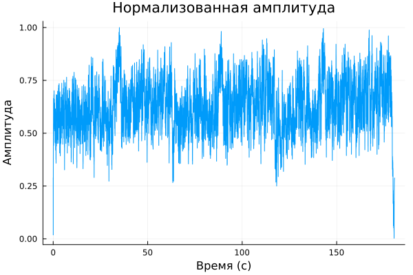
# Plotting a graph
gr()
plot(t, normalized_audio, title="Normalized amplitude", xlabel="Time (s)", ylabel="The amplitude", legend=false)

Variables t and normalized_audio they are loaded into the model using the block Табличная функция одной переменной in the subsystem Звуковой сигнал. After connecting the garland to the KPM RHYTHM and processing the audio file, the following result is obtained:
Гирлянда.gif

Full video of the work: