Modeling and analysis of AFE active rectifier operation

The example is devoted to modeling and analyzing the operation of an AFE (Active Front End) rectifier, including the study of its control algorithms, energy consumption and recovery modes. Based on Engee modeling, the key advantages of AFE are demonstrated: maintaining a power factor close to 1, reducing harmonic distortion of current to 5.8%, and voltage stabilization in the DC link. The results of the work are relevant for developers of power electronics systems, energy-efficient transport and industrial electric drives, where modern approaches to energy flow management and minimizing the impact on the network are required.

Introduction

AFE Rectifier (Active Front End) is an active electronic device designed to convert alternating current to direct current with a high power factor and minimal harmonic distortion. Its creation is associated with the development of power electronics since the 1980s, when Siemens, ABB, Danfoss and others began to implement IGBT and digital control systems. Unlike passive diode rectifiers, AFE uses IGBTs operating "on the grid", which ensures the bidirectionality of the converter: not only to consume energy from the grid, but also to return it back, for example, during regenerative braking.

AFE rectifiers are used in industrial electric drives, renewable energy systems, transportation (electric trains, subways, electric buses) and energy-intensive industries (rolling mills, data processing centers). For example, in subways, AFE provides braking energy recovery to the grid, reducing overall energy consumption. The key advantages of such rectifiers are high efficiency, compactness, reduced interference in the network and the ability to work with unstable voltage. These features make them indispensable in modern systems where intelligent energy management and environmental sustainability are required.

The example model

Model Active_front_end.engee The model considered in this example is recreated from an analog model Active_front_end.slx [1].

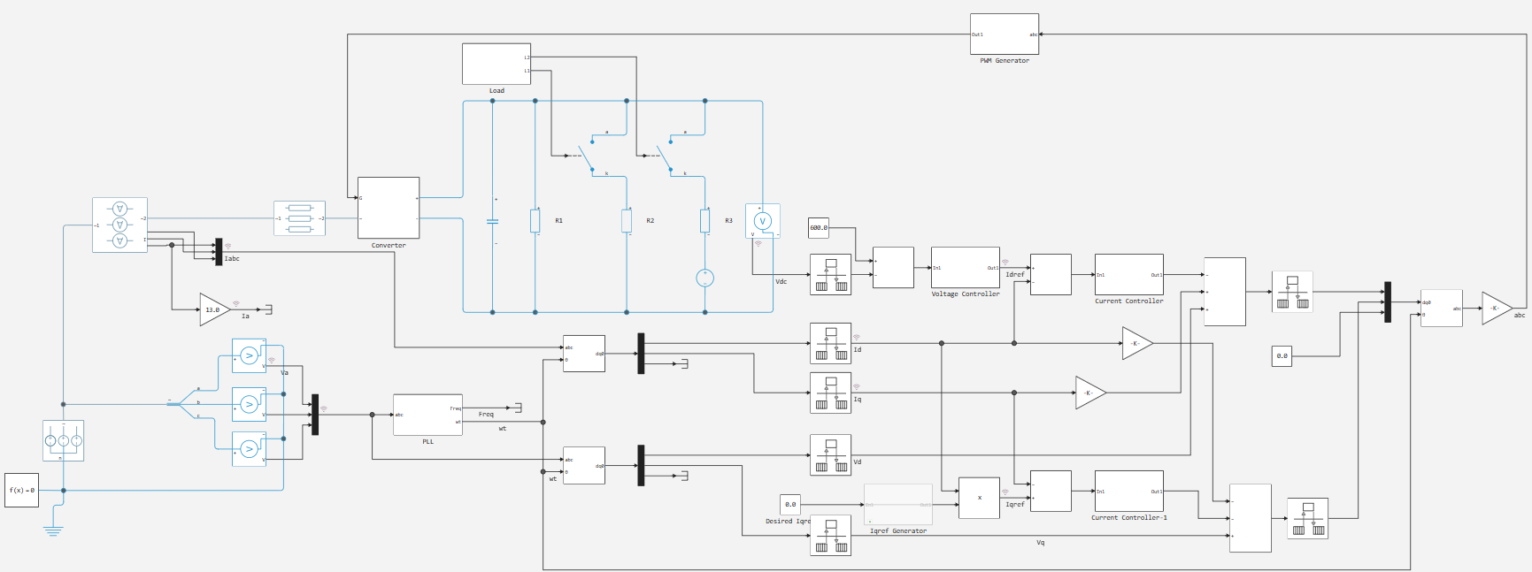
The power unit consists of the following elements.

Three-phase voltage source .
Phase voltage and current measurement units.
Cable line with resistance and the inductance .
Bridge three-phase converter Converter On NPN-IGBT with reverse diodes, the upper switches are installed by collectors in a three-phase network, and the reverse diodes act as a rectifier kit.
A DC link capacitor with a capacity of .
The minimum active load in the DC link is a resistor with resistance .
The connected active load in the DC link is a resistor with a resistance .
Plug-in anti-EMF in a direct current link with a value of , and a resistor with resistance - simulated braking.
A voltmeter in the direct current link.

Load it is activated at the moment model time, turns off in . A circuit with an anti-EMF is switched to .

The AFE algorithm operates in all modes of operation of the rectifier.

Description of the AFE operation principle

IGBT converter (Converter) receive PWM control signals from the PWM generator module (PWM Generator). The PWM reference signal is triangular with a frequency of . The set signals of the PWM generator are phase voltages in a three-phase coordinate system :

In turn, obtained by inverse Park-Gorev transformation from

where - set stresses in the rotating coordinate system ,
- the angle of rotation of the rotating coordinate system, calculated using phase frequency auto-tuning (PLL) in the block PLL.

In turn, these components are defined by the following expressions:

Here:

- the basic harmonic of the supply voltage;
- measured stresses in the rotating coordinate system ;
- measured phase currents in a rotating coordinate system ;
- output voltage of PI current regulators Current Controller in a rotating coordinate system ;

Voltage and currents obtained using the [Park-Gorev direct conversion] blocks1 from the measured phase currents and voltages and :

PI current regulators Current Controller the difference between the measured and set current signals in the rotating coordinate system is obtained :

Projection of a given current onto an axis , - the result of regulation of the PI voltage regulator Voltage Controller. It receives the difference between the measured and set voltage values in the DC link:

Projection of a given current onto an axis , is set to equal for the formation of

The AFE control system presented above reproduces these ratios in the form of a block diagram.

Simulation

Using software control, we will execute the example model and write the simulation results into a variable simout.

модель = engee.load("/user/start/examples/power_systems/active_front_end_rectifier/Active_front_end.engee", force = true);     # Загружаем модель
engee.run(модель);                                           # Выполняем модель и сохраняем данные

After completing the model, we will close it and proceed to signal analysis.

engee.close(модель; force=true);

Analysis of recorded signals

From the recorded signals of the model, we will select the signals of the simulation time, current and voltage of phase A, and voltage in the DC link:

t = simout["Active_front_end/Va"].time;
Va = simout["Active_front_end/Va"].value;
Ia = simout["Active_front_end/Ia"].value;
Vdc = simout["Active_front_end/Vdc"].value;

We will output phase A current and voltage waveforms for different AFE operating modes: consumption with normal load, consumption with increased load and recovery.

using Plots; gr()

start = Int(1e6÷5*0.5);
start_load = Int(1e6÷5);
start_recup = Int(1e6÷5*3); 
stop = Int(1e6÷5/50*5);

usual = start:start+stop
load = start_load:start_load+stop
recup = start_recup:start_recup+stop;

plot_usual = plot(t[usual], [Ia[usual], Va[usual]]; label=["Ia⋅13, А" "Va, В"], title = "Обычная нагрузка")
plot_load = plot(t[load], [Ia[load], Va[load]]; label=["Ia⋅13, А" "Va, В"], title = "Повышенная нагрузка")
plot_recup = plot(t[recup], [Ia[recup], Va[recup]]; label=["Ia⋅13, А" "Va, В"], title = "Рекуперация")

plot(plot_usual, plot_load, plot_recup;
     size=(1200,300), legend = :topright, xlabel = "Время, с", ylabel = "Напряжение, ток", layout=(1,3))

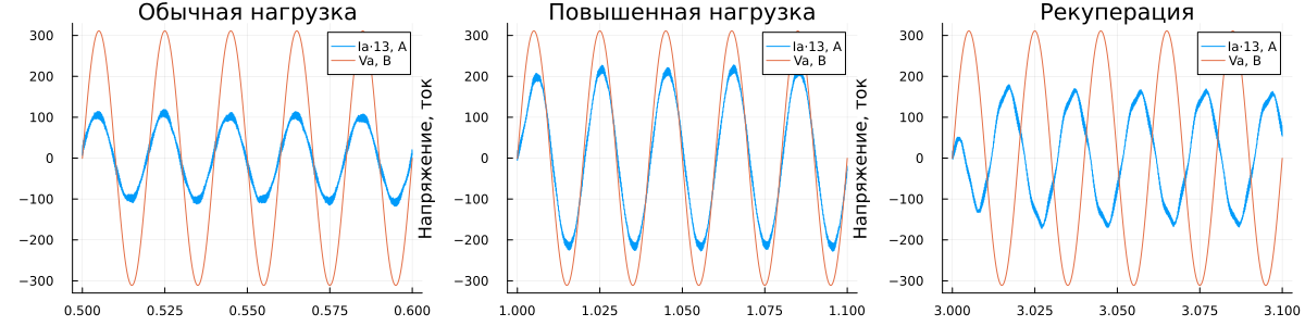
As can be seen from these waveforms, current and voltage are in phase in consumption mode, the shape of the consumed/generated current is close to sinusoidal, and in recovery mode, the phases of current and voltage are inverted. The latter means that AFE provides the recovery of braking energy into the network (which is simulated by switching on the anti-EMF in the DC link).

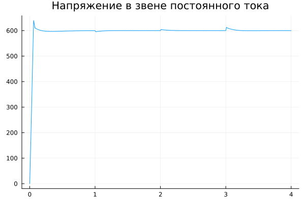
Based on the voltage graph in the DC link, which is shown below, it can be concluded that in various AFE operating modes, the voltage level is stabilized and equal to the set value .

gr(); plot(t[1:2000:end], Vdc[1:2000:end]; legend=:none, title = "Напряжение в звене постоянного тока")

Power factor analysis

We will install and connect the necessary libraries for analysis

import Pkg; Pkg.add(["FFTW", "LinearAlgebra"]);
using FFTW, LinearAlgebra;

In addition to maintaining voltage in the DC link and ensuring energy recovery to the grid, the AFE rectifier compensates for reactive power consumption by increasing the power factor. up to almost 1. Based on the data obtained (voltage and current of phase A), we will calculate and analyze the power factor for each voltage period.

# Подключим функцию расчёта коэффициента мощности для каждого периода входных векторов тока и напряжения
include("/user/start/examples/power_systems/active_front_end_rectifier/pf_calculation.jl");
# Расчет коэффициентов
коэффициенты_мощности = calculate_power_factor(Vector(Va), Vector(Ia));

# Построим интерактивный график коэффициента мощности
plotlyjs();
plot(0:0.02:3.98, коэффициенты_мощности;
    legend=:none, title="Коэффициент мощности", ylabel="cos(ϕ), о.е.")

From the resulting graph of the power factor, we can judge the following:

in the mode of energy consumption from the grid AFE provides regardless of the load level;
in the mode of energy recovery to the grid AFE provides ;

Analysis of harmonic distortion during AFE operation

Another indisputable advantage of using an active AFE rectifier is the reduction of harmonic distortion of current both in consumption mode and during recovery. From the current waveforms above, it can be seen that in the recovery mode, the signal is larger than in the consumption modes, and differs in shape from a sine wave. In addition, during certain periods of the carrier frequency, harmonic distortion will be more pronounced than during the entire operating mode. Therefore, to estimate the maximum value of the harmonic distortion coefficient (THD) of current and voltage, we will take a section with a duration of one period of the base harmonic of the supply voltage. in recovery mode.

# Подключим функцию для расчёта THD и гармонического спектра
# Скрипт также устанавливает и подключает требуемые библиотеки (FFTW.jl, LinearAlgebra.jl)
include("/user/start/examples/power_systems/active_front_end_rectifier/thd_calculation.jl");

# Зададим начальные условия
start_recup = Int(1e6÷5*3.02);  # Начальная точка анализа
stop = Int(1e6÷5*3.04);         # Конечная точка анализа

sample_rate = Int(1e6÷5)        # Частота дискретизации, Гц
f_base = 50;                    # Частота базовой гармоники, Гц
n_max = 40;                     # Наибольший порядок искажающей гармоники

# Получим результаты анализа THD и гармонических спектров
result_Ia = calculate_thd(Ia[start_recup:stop], sample_rate, n_max, f_base);
result_Va = calculate_thd(Va[start_recup:stop], sample_rate, n_max, f_base);

# Построим гармонические спектры тока и напряжения, выведем значения THD
gr();

let
    # График гармонического спектра тока
    plot(result_Ia.frequencies, result_Ia.amplitudes, 
        label="Спектр тока", linewidth=2)

    # График гармонического спектра напряжения
    plot!(result_Va.frequencies, result_Va.amplitudes, 
        label="Спектр напряжения", linewidth=1,
        seriestype=:path, linestyle=:dash, color=:black)

    # Маркер амплитуды базовой гармоники
    scatter!([result_Ia.frequencies[result_Ia.fundamental_idx]], 
            [result_Ia.amplitudes[result_Ia.fundamental_idx]],
            label="Базовая гармоника", markersize=4, color=:red)
    vline!([result_Ia.frequencies[result_Ia.fundamental_idx]], 
            linestyle=:dash, color=:gray, label=:none)

    # Маркеры амплитуд гармоник высших порядков
    if !isempty(result_Ia.frequencies[result_Ia.harmonic_indices])
        scatter!(result_Ia.frequencies[result_Ia.harmonic_indices], 
                result_Ia.amplitudes[result_Ia.harmonic_indices],
                label="Высшие гармоники", markersize=4, color=:green)
        vline!(result_Ia.frequencies[result_Ia.harmonic_indices],
              linestyle=:dash, color=:gray, label=:none)
    end
    
    # Настройки отображения
    xlims!(0, n_max)
    xticks!(1:2:n_max)
    display(plot!(yscale=:log; xlabel="Частота, (Гц)", ylabel="Амплитуда, log(A)",
            title="Гармонический анализ", legend=:bottom,))

    # Вывод значений суммарных гармонических искажений напряжения и тока
    println("THD_v: ", round(result_Va.thd, digits=2), " %")
    println("THD_i: ", round(result_Ia.thd, digits=2), " %")
end

THD_v: 0.01 %
THD_i: 5.8 %

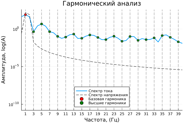
The representation of the harmonic spectrum on a logarithmic amplitude scale is not classical, but it provides the most detailed visual representation of the spectral composition of the analyzed signal. From the data obtained, we can judge the following:

The total level of harmonic distortion of the current Consequently, AFE fully copes with the reduction of harmonic distortion of the current from an uncontrolled rectifier.
The harmonics most pronounced on the current spectrum belong to the orders of , where - pulsation of the rectifier circuit.

Conclusion

In the example, the AFE rectifier operation was simulated using Engee, which confirmed the device's ability to maintain a power factor close to 1 and reduce harmonic current distortion by up to 5.8% even in recovery mode. It is shown that the system stably maintains the voltage in the DC link at a given level (for example, 800 V) under variable loads, demonstrating the effectiveness of bidirectional energy management. The results confirm that AFE significantly reduces reactive power and electromagnetic interference, which is critical for energy-intensive facilities (metro, industrial drives).

Used sources

Ricardo Palma (2025). Active front end rectifier (https://www.mathworks.com/matlabcentral/fileexchange/63357-active-front-end-rectifier), MATLAB Central File Exchange. Retrieved April 29, 2025.