Detection at a constant probability of false alarm (PVLT)
This example examines the detection with a constant probability of false alarm (HLT) and shows how to use CFARDetector and CFARDetector2D from the EngeePhased library to implement the HLT detection algorithm.
Used fuctions
Pkg.add(["DSP"])
include("$(@__DIR__)/functions.jl");
Introduction
One of the important tasks that the radar system performs is target detection. The detection procedure itself is quite simple. It compares the signal with a threshold value. Therefore, the real job of detection is to determine the appropriate threshold. In general, the threshold is a function of both the probability of correct detection and the probability of a false alarm.
In many phased array systems, due to the costs associated with false detection, it is desirable to have a detection threshold that not only maximizes the probability of correct detection, but also keeps the probability of false alarm below a preset level.
There is an extensive literature on how to determine the detection threshold. Readers may be interested in examples of signal detection in white Gaussian noise and signal detection from several samples, where some well-known results are presented. However, all these classical results are based on theoretical probabilities and are limited to white Gaussian noise with a known variance (power). In real devices, noise is often colored, and its power is unknown.
The CFAR algorithm solves these problems. When it is required to detect a specific cell, often referred to as a test cell (CUT), the noise power is estimated from neighboring cells. In this case, the detection threshold (T) is determined as follows:
where - evaluation noise power, - scale (threshold) coefficient
It can be seen from the equation that the threshold adapts to the data. It can be shown that with an appropriate threshold coefficient α, the resulting probability of a false alarm can be maintained at a constant level, hence the name PVLT.
Cell averaging. Detection with PVLT
The cell-averaged CFAR detector is probably the most widely used CFAR detector. It is also used as a base comparison for other CFAR methods. In a cell-averaged CFAR detector, noise samples are extracted from the leading and lagging cells (so-called training cells) around the CUT. The noise estimate can be calculated as:
 where $N$ - the number of training cells, and $x_m$ - selection in each training cell.
If is the output of the quadratic law detector, then represents the estimated noise power. In general, the number of leading and lagging training cells is the same. Security cells are located next to the CUT, both in front and behind it. The purpose of these protective cells is to avoid leakage of signal components into the training cell, which can negatively affect the noise assessment.
The following figure shows the relationship between these cells for case 1-D.
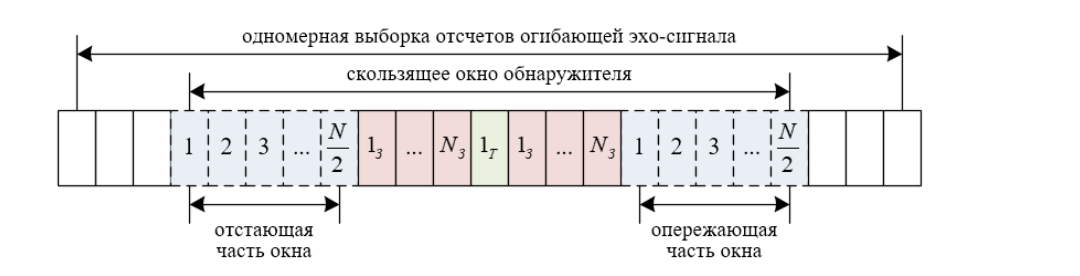
In the above cell-averaged CFAR detector, assuming that the data in the detector comes from a single pulse, i.e. without pulse integration, the threshold coefficient can be written as:
where - the required probability of a false alarm.
CFAR detection using an automatic threshold coefficient
In the rest of this example, we will show how to use EngeePhased to perform cell-averaged CFAR detection. For simplicity and without loss of generality, we still assume that the noise is white Gaussian. This allows us to compare CFAR with classical detection theory.
We can create a CFAR detector using the following command:
cfar = EngeePhased.CFARDetector(NumTrainingCells=20,NumGuardCells=2);
In this detector, we use 20 training and 2 protective cells. This means that there are 10 training cells and 1 safety cell on each side of the CUT. As mentioned above, if we assume that the signal comes from a detector with a quadratic law without pulse integration, the threshold can be calculated based on the number of training cells and the desired probability of a false alarm. Assuming that the desired false alarm probability is 0.001, we can configure the CFAR detector as follows so that this calculation can be performed.
exp_pfa = 1e-3 # the probability of a false alarm
cfar.ThresholdFactor = "Auto" # threshold detection algorithm (Automatic)
cfar.ProbabilityFalseAlarm = exp_pfa;
The configured CFAR detector is shown below.
cfar
Now we will simulate the input data. Since we want to show that the CFAR detector can keep the false alarm level below a certain value, we will simply simulate the noise in these cells. Here are the settings:
- The data sequence is 23 samples long, and the CUT is cell 12. This leaves 10 training cells and 1 safety cell on each side of the CUT.
- The false alarm rate is calculated using 100,000 Monte Carlo tests.
rng = MersenneTwister(20)
npower = db2pow(-10);  # The SNR task is 10dB

Ntrials = Int(1e5);
Ncells = 23;
CUTIdx = 12;

# The noise model after the quadratic detector
rsamp = randn(rng,Ncells,Ntrials)+1im*randn(rng,Ncells,Ntrials);
x = abs.(sqrt.(npower/2)*rsamp).^2;
To perform detection, pass the data through the detector. In this example, there is only one CUT, so the output is a logical vector containing the detection result for all tests. If the result is true, it means that the target is present in the corresponding test. In our example, all the detections are false alarms, since we only pass through noise. As a result, the false alarm rate can be calculated based on the number of false alarms and the number of trials.
x_detected = cfar(x,CUTIdx);
act_pfa = sum(x_detected)/Ntrials;
println("act_pfa = $(act_pfa)")
The result shows that the resulting probability of a false alarm is 0.001, as we assumed.
Detecting CFAR using a custom threshold coefficient
As explained in the previous part of this example, there are only a few cases where the CFAR detector can automatically calculate the appropriate threshold coefficient. For example, in the previous scenario, if we use 10-pulse incoherent integration before receiving data to the detector, the automatic threshold will no longer be able to provide the desired false alarm rate.:
npower = db2pow(-10);  # The SNR value is 10 dB
xn = 0;
for m = 1:10
    rsamp = randn(rng,Ncells,Ntrials) .+ 1im*randn(rng,Ncells,Ntrials);
    xn = xn .+ abs.(sqrt.(npower/2)*rsamp).^2 # incoherent accumulation
end
x_detected = cfar(xn,CUTIdx);
act_pfa = sum(x_detected)/Ntrials
println("act_pfa = $act_pfa")
It may be confusing why we believe that a false alarm rate of 0 is worse than a false alarm rate of 0.001. After all, isn't a false alarm rate of 0 a great thing? The answer to this question lies in the fact that as the probability of a false alarm decreases, so does the probability of detection. In this case, since the true probability of a false alarm is much lower than the acceptable value, the detection threshold is set too high. The same detection probability can be achieved with the desired false alarm probability at a lower cost; for example, with lower transmitter power.
In most cases, the threshold coefficient must be determined depending on the specific environment and system configuration. We can configure the CFAR detector to use a custom threshold coefficient, as shown below.
release!(cfar);
cfar.ThresholdFactor = "Custom";
Continuing to look at the example of pulse integration and using empirical data, we found that a custom threshold factor of 2.35 can be used to achieve the desired false alarm rate. Using this threshold, we can see that the false alarm coefficient obtained corresponds to the expected value.
cfar.CustomThresholdFactor = 2.35;
x_detected = cfar(xn,CUTIdx);
act_pfa = sum(x_detected)/Ntrials
println("act_pfa = $act_pfa")
CFAR detection threshold
CFAR detection occurs when the input signal level in a cell exceeds a threshold level. The threshold level for each cell depends on the threshold coefficient and the noise power in that cell obtained from the training cells. To maintain a constant level of false alarms, the detection threshold will increase or decrease in proportion to the noise power in the training cells. Configure the CFAR detector to output the threshold used for each detection using the ThresholdOutputPort property. We will set the automatic calculation mode for the threshold coefficient and 200 training cells.
release!(cfar);
cfar.ThresholdOutputPort = true;
cfar.ThresholdFactor = "Auto";
cfar.NumTrainingCells = 200;
Then we will generate a quadratic input signal with increasing noise power.
Npoints = 10_000;
rsamp = randn(rng,Npoints).+1im*randn(rng,Npoints);
ramp = Vector(range(1,10;length=Npoints));
xRamp = abs.(sqrt.(npower*ramp./2).*rsamp).^2;
Calculate the detections and thresholds for all cells in the signal.
x_detected,th = cfar(xRamp,Vector(1:length(xRamp)));
Then compare the CFAR threshold value with the input signal.
gr()
plot(1:length(xRamp),xRamp,label="The signal",line=(2,:blue,:sticks))
plot!(1:length(xRamp),th,label="Doorstep")
scatter!(findall(x_detected[:] .> 0),xRamp[findall(x_detected[:] .> 0)],label="Detection",marker=(:circle,4,:yellow))
xlabel!("Time counts")
ylabel!("The amplitude",legend=:topleft)
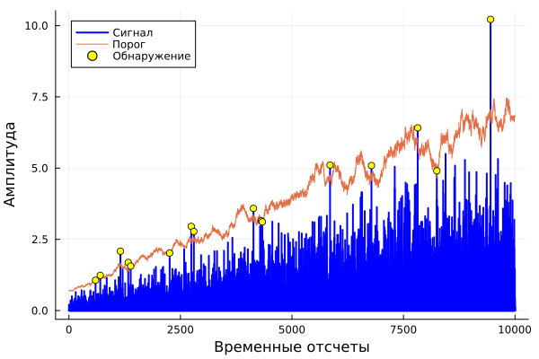
Here, the threshold increases with increasing noise power in the signal to maintain a constant false alarm level. Detection occurs where the signal strength exceeds a threshold value.
Comparison of CFAR with the classical Neiman-Pearson detector
In this section, we will compare the performance of the CFAR detector with classical detection theory using the Neumann-Pearson principle. Going back to the first example and assuming that the true noise power is known, the theoretical threshold can be calculated as
T_ideal = npower*db2pow(npwgnthresh(exp_pfa));
The false alarm coefficient of this classic Neiman-Pearson detector can be calculated using this theoretical threshold.
act_Pfa_np = sum(x[CUTIdx,:] .> T_ideal)/Ntrials
println("act_Pfa_np = $act_Pfa_np")
Since we know the noise power, the classical detection theory also allows us to obtain the desired false alarm coefficient. The false alarm rate achieved by the CFAR detector is similar.
release!(cfar);
cfar.ThresholdOutputPort = false;
cfar.NumTrainingCells = 20;
x_detected = cfar(x,CUTIdx);
act_pfa = sum(x_detected)/Ntrials
println("act_pfa = $act_pfa")
Next, let's assume that both detectors are deployed in the field and the noise power is 1 dB higher than expected. In this case, if we use a theoretical threshold, the resulting probability of a false alarm will be four times greater than we want.
npower = db2pow(-9); # Assume 9dB SNR ratio
rsamp = randn(rng,Ncells,Ntrials).+1im*randn(rng,Ncells,Ntrials);
x = abs.(sqrt.(npower/2)*rsamp).^2;
act_Pfa_np = sum(x[CUTIdx,:] .> T_ideal)/Ntrials
println("act_Pfa_np = $act_Pfa_np")
On the contrary, it does not affect the operation of the CFAR detector.
x_detected = cfar(x,CUTIdx);
act_pfa = sum(x_detected)/Ntrials
println("act_pfa = $act_pfa")
Thus, the CFAR detector is resistant to noise power uncertainty and is better suited for field applications.
Finally, we use CFAR detection in the presence of color noise. First, we apply the classical detection threshold to the data.
npower = db2pow(-10);
fcoeff = [-0.00057693500095478268512028119374691, 0.0004446399942713034555974438433168, 0.023749844987587823141872434007382, 0.10475951999236174372320817838045, 0.22682709001336692766770397611253, 0.2895916800267339108465591834829, 0.22682709001336692766770397611253, 0.10475951999236174372320817838045, 0.023749844987587819672425482053768, 0.0004446399942713034555974438433168, -0.00057693500095478268512028119374691]
x = abs.(sqrt(npower/2)*filt(fcoeff,1,rsamp)).^2;   # colored noise
act_Pfa_np = sum(x[CUTIdx,:] .> T_ideal)/Ntrials
println("act_Pfa_np = $act_Pfa_np")
Please note that the false alarm coefficient obtained may not meet the requirements. However, by using a CFAR detector with a custom threshold coefficient, we can obtain the desired false alarm coefficient.
release!(cfar);
cfar.ThresholdFactor = "Custom";
cfar.CustomThresholdFactor = 12.85;
x_detected = cfar(x,CUTIdx);
act_pfa = sum(x_detected)/Ntrials
println("act_pfa = $act_pfa")
CFAR detection by range-Doppler portrait
In the previous sections, the noise estimate was calculated based on the training cells leading and lagging behind the CUT in one dimension. We can also perform CFAR detection on images. The cells correspond to pixels in the images, and the protective and training cells are arranged in stripes around the CUT. The detection threshold is calculated from the cells in the rectangular learning band around the CUT.
In the figure above, the size of the protective strip is [2 2], and the size of the training strip is [4 3]. The size indexes indicate the number of cells on each side of the CUT in the row and column, respectively. The size of the protective strip can also be defined as 2, since its size is the same in rows and columns.
Next, create a two-dimensional CFAR detector. Use the 1e-5 false alarm probability and specify the size of the 5-cell protective strip and the size of the 10-cell training strip.
cfar2D = EngeePhased.CFARDetector2D(GuardBandSize=5,TrainingBandSize=10,
  ProbabilityFalseAlarm=1e-5);
Then download and build the range Doppler image. The image includes returns from two stationary targets and one target moving away from the radar.
hrdresp = EngeePhased.RangeDopplerResponse(
    DopplerFFTLengthSource="Property",
    DopplerFFTLength=RangeDopplerEx_MF_NFFTDOP,
    SampleRate=RangeDopplerEx_MF_Fs);
resp,rng_grid,dop_grid = step!(hrdresp,RangeDopplerEx_MF_X,RangeDopplerEx_MF_Coeff);

# Adding white noise

npow = db2amp(-95);
resp = resp .+ npow/sqrt(2)*(randn(rng,size(resp)) .+ 1im*randn(rng,size(resp)))

plot_1 = heatmap(dop_grid,rng_grid,mag2db.(abs.(resp)),colorbar=false,margin=5Plots.mm,
    color = :rainbow1, titlefont = font(12,"Computer Modern"),
    guidefont = font(10,"Computer Modern"))
resp = abs.(resp).^2;
xlabel!("Doppler Frequency, Hz")
ylabel!("Range, m")
title!("Range-Doppler portrait")
rangeIndx = map(x -> x[1],(findmin(abs.(rng_grid[:] .- [1000 4000]);dims=1)[2]))
dopplerIndx = map(x -> x[1],(findmin(abs.(dop_grid[:] .- [-1e4 1e4]);dims=1)[2]))
columnInds,rowInds = meshgrid(dopplerIndx[1]:dopplerIndx[2],rangeIndx[1]:rangeIndx[2]);
CUTIdx = permutedims([rowInds[:] columnInds[:]])
Calculate the detection result for each tested cell. In this example, each pixel in the search area is a cell. Build a map of the detection results for the range-Doppler image.
detections = cfar2D(resp,CUTIdx)
detectionMap = zeros(size(resp))
detectionMap[rangeIndx[1]:rangeIndx[2],dopplerIndx[1]:dopplerIndx[2]] =
  reshape(float(detections),rangeIndx[2]-rangeIndx[1]+1,dopplerIndx[2]-dopplerIndx[1]+1);
heatmap(dop_grid,rng_grid,mag2db.(abs.(detectionMap .+ 1eps(1.))),colorbar=false,c = :imola,
  titlefont = font(12,"Computer Modern"),guidefont = font(10,"Computer Modern"),margin=5Plots.mm)
xlabel!("Doppler Frequency, Hz")
ylabel!("Range, m")
title!("Range-Doppler portrait after CFAR detection")
Three objects have been detected. As an input signal for cfar2D, you can also provide a cube of rangefinder Doppler image data over time, and the detection will be calculated in one step.
Conclusion
In this example, we have presented the basic concepts underlying CFAR detectors. In particular, we looked at how to use the EngeePhased toolkit to perform a cell-averaged CFAR detector on signals and rangefinder Doppler images. A comparison of the characteristics of a CFAR detector with cell averaging and a detector with a theoretically calculated threshold clearly shows that the CFAR detector is more suitable for real field conditions.