A system model of a single-position radar system with a single purpose
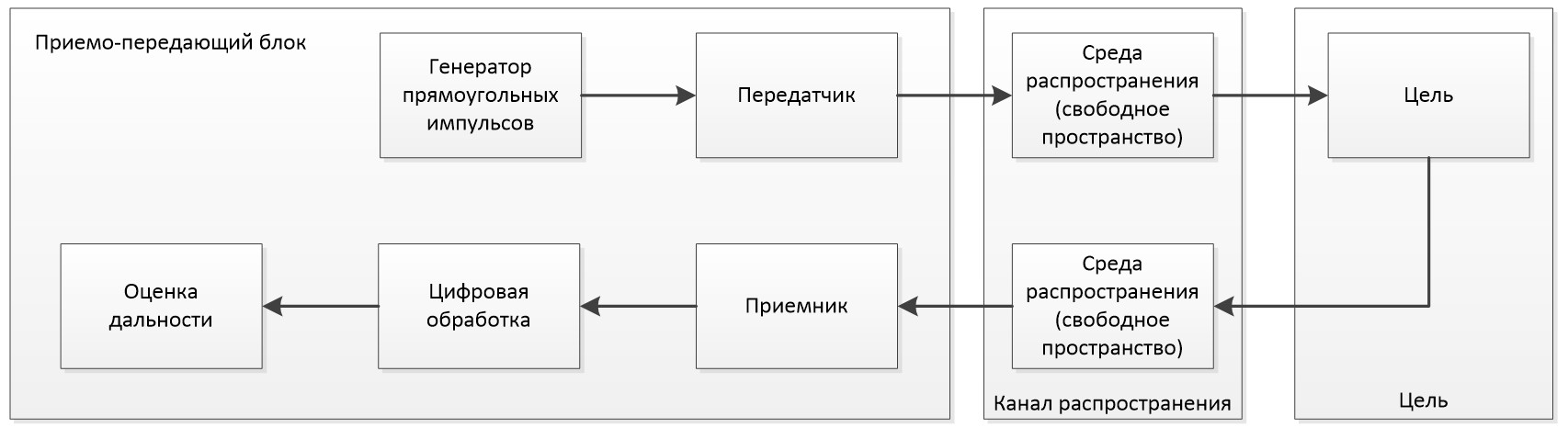
This model demonstrates the operation of a simple single-position radar system.
The special feature of the model is that the radar transmitter and receiver do not contain an antenna array. Thus, the antenna is equivalent to a simple isotropic element.
A sequence of rectangular pulses is used as a probing signal, which are amplified in the transmitter.
Then, from the output of the transmitter, the signal propagates to the target through the free space. The reflected signal is sent to the receiver.
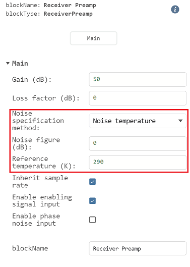
The receiver amplifies the signal and also adds its own noise.
A matched filter is used as the processing unit, and propagation losses are compensated by gain control.
The final stage of processing is incoherent accumulation. The model's operation scheme is shown in the figure below.
Digital processing consists of the following elements:

Next, we will connect libraries and files with functions that we will need during the processing of data recorded from the model and during the initialization of model parameters.
cd( @__DIR__ )
# Loading the initialization function of the model
include( "initParamRadar.jl" );
Initialization of the model parameters.
paramRadar = calcParamRadar();
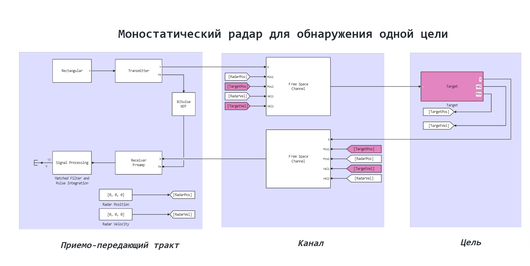
Based on the block diagram, we have developed the radar model shown in the figure below.
Let's run the model through a custom function.
modelName = "MonostaticRadar";
model = modelName in [m.name for m in engee.get_all_models()] ? engee.open( modelName ) : engee.load( "$(@__DIR__)/$(modelName).engee");
results =  engee.run( modelName,verbose=true );
Please note: the signal on the receiver has temperature noise.
Let's open the results and build a peak.
file_Rectangular_out = reduce(hcat, results["Y"].value)
R = paramRadar.metersPerSample .* (0:size(file_Rectangular_out, 1) - 1) .+ paramRadar.rangeOffset

plot( R,file_Rectangular_out[:,2]*1e6,label="",title="Correlation response at the output of the model",
    color=:red,lw=2,xlabel="Range, m",ylabel="Power, MCW")
Conclusion
We have reviewed the operation of a simple single-position radar system. The final graph of the integrator's output shows that the system has found a peak, that is, it was able to detect an object at a distance of 2000 meters. This means that this radar method is working correctly.