A two-purpose bistatic radar system model
In the example, let's look at modeling a bistatic radar system with two objectives. The transmitter and receiver of the bistatic radar are located differently and move along different trajectories.
1. Description of the model structure
Let's take a closer look at the functional structure of the model:
- Source (Linear FM): a continuous signal with linear frequency modulation is used as a probing signal (the band is 3 MHz, which corresponds to 50 meters of range resolution);
- Radar Transmitter: Amplifies the pulse and simulates the motion of the transmitter;
- Distribution Environment (FreeSpace): The signal propagates to the targets and back to the receiver, undergoing attenuation proportional to the distance to the target;
- Target (Radar Targets): Reflects the incident signal and simulates the movement of both targets;
- Receiver (Radar Receiver): Receives the reflected signal from the target, adds receiver noise and simulates movement;
- Filtering (Range Doppler Processing): The processing unit uses a buffer to accumulate 64 pulses and the processor performs consistent filtering to estimate range and FFT to estimate Doppler shift (speed) ;
The model's operation scheme is shown in the figure below.
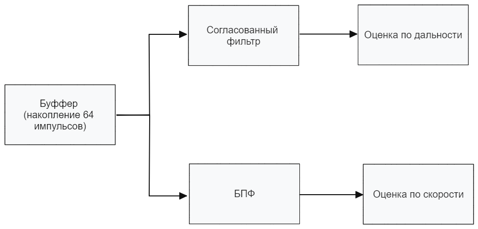
Digital processing consists of the following elements:
.png)
The radar model is shown in the figure below.
2. Initialization of input parameters
To initialize the input parameters of the model, we will connect the file "Parambistic.jl". If you need to change the parameter values, then open this file and edit the necessary parameters.
include("$(@__DIR__)/ParamBistatic.jl")

paramBistatic = calc_param_BistaticRadar();
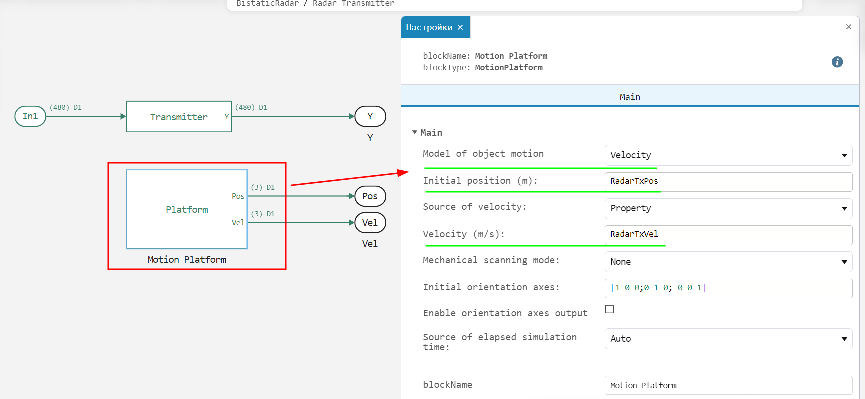
In the model, the receiver and the transmitter are separated and move along different trajectories. 3 motion models are supported: uniform, equidistant and custom (the trajectory is set point-by-point). An example of setting a uniform motion of the transmitter is given below:
.png)
3. Launching the model
function run_model( name_model, path_to_folder ) # defining a function for running the model
    Path = path_to_folder * "/" * name_model * ".engee"
    if name_model in [m.name for m in engee.get_all_models()] # Checking the condition for loading a model into the kernel
        model = engee.open( name_model ) # Open the model
        model_output = engee.run( model, verbose=true ); # Launch the model
    else
        model = engee.load( Path, force=true ) # Upload a model
        model_output = engee.run( model, verbose=true ); # Launch the model
        engee.close( name_model, force=true ); # Close the model
    end
    return model_output
end;
out = run_model( "BistaticRadar", @__DIR__); # Launch the model
4. Reading the output data
We calculate the necessary output from the out variable (in our case, "out_bistatic"):
out_bistatic_engee = zeros(ComplexF64,size(out["out_bistatic"].value[1],1),size(out["out_bistatic"].value[2],2),length(out["out_bistatic"].value))
[out_bistatic_engee[:,:,i] = collect(out["out_bistatic"].value[i]) for i in eachindex(out["out_bistatic"].value)];
5. Displaying the results
Let's build the system's response based on speed and range, obtained in the previous paragraph.:
abs_out_map = abs.(out_bistatic_engee[:,:,2]).+eps(1.0)
range_doppler_map =  10log10.(abs.(abs_out_map).^2)
x_speed = range(-5000,5000;length = length(range_doppler_map[1,:]))
y_range = range(0,45;length = length(range_doppler_map[:,1]))
Plots.heatmap(x_speed, y_range, range_doppler_map,ylabel="Range, km ",
    xlabel="Speed km/h", title="Map of Doppler and time delays", colorbar_title="Power, dBW",
    color=:viridis,size = (600,400), margin = 5*Plots.mm)
Conclusion
In the example, the operation of a bistatic radar system with two objectives was considered. As a result of the radar operation, a map of Doppler responses (in terms of speed) and time delays (range) was built, which was used to determine the position and speeds of the two targets.