Object tracking using GNN

In the modern world, object tracking tasks have wide applications, from autonomous vehicles and video surveillance systems to radar and sensor monitoring.
One of the key problems in this area has been the association of measurements with tracks, especially in conditions of uncertainty, noise, and possible intersections of trajectories.

We will consider the implementation of the classic GNN tracking algorithm.

The presented code includes the following steps.

Modeling the movement of objects along hyperbolic trajectories.
Implementation of the Kalman filter for predicting and updating track states.
Visualization of the results in the form of an animated graph.

The main goal is to demonstrate the effectiveness of an algorithm for processing noisy measurements and constructing trajectories of moving objects, in this case objects moving along hyperbolic trajectories.

Next, let's move on to the algorithm and start by declaring data structures and constants for the object tracking system.

Track is a modifiable structure that stores the state of an object (coordinates, velocity), the covariance matrix (uncertainty), the age of the track, the number of missed measurements, and the history of states for visualization.
Detection is an immutable structure for storing measurements (coordinates and time).
A 2×4 observation matrix H that extracts positional components (x,y) from the state vector.

These structures form the basis for the implementation of the algorithm.

using LinearAlgebra

# Changeable track structure
mutable struct Track
    state::Vector{Float64}     # The state vector
    covariance::Matrix{Float64} # The covariance matrix
    age::Int                   # Track age (number of updates)
    missed::Int                # Number of missed measurements
    history::Vector{Vector{Float64}} # History of states for rendering
end

# Adding history to the Track constructor
Track(state, covariance, age, missed) = Track(state, covariance, age, missed, [copy(state)])

# Dimension: [x, y, timestamp]
struct Detection
    position::Vector{Float64}
    time::Float64
end

const H = [1 0 0 0; 0 1 0 0];  # The observation matrix

Next, let's look at the implementation of the Kalman filter for tracking.

predict! Updates the track status based on the constant velocity (CV) model, predicting the new position and increasing uncertainty (covariance).
update! Adjusts the track state by measurement using the Kalman gain matrix (K), reducing uncertainty and maintaining a history of changes.

# Track condition prediction function
function predict!(track::Track, dt::Float64)
    F = [1 0 dt 0; 0 1 0 dt; 0 0 1 0; 0 0 0 1]  # Transition Matrix (CV)
    track.state = F * track.state
    track.covariance = F * track.covariance * F' + diagm([0.1, 0.1, 0.01, 0.01])
    return track
end

# Track update function based on measurement
function update!(track::Track, detection::Detection)
    y = detection.position - H * track.state
    S = H * track.covariance * H' + diagm([0.5, 0.5])
    K = track.covariance * H' / S
    track.state += K * y
    track.covariance = (I - K * H) * track.covariance
    track.age += 1
    track.missed = 0
    push!(track.history, copy(track.state)) # Saving the history
    return track
end

[ Info: Starting sender/receiver loops

update! (generic function with 1 method)

Let's move on to the tracking algorithm function. Global Nearest Neighbor (GNN) is a simple method based on greedily matching measurements to nearby tracks. In our code, the trackerGNN function implements the GNN algorithm for matching tracks and measurements. The algorithm itself consists of the following parts.

Prediction: Copies and predicts new states of all tracks (predict!).
Calculation of distances: builds a matrix of distances between tracks and measurements based on the Mahalanobis statistical distance.
Greedy matching: Finds track-dimension pairs with a minimum distance by checking the threshold and excludes tracks/dimensions that have already been matched.
Update and Filtering: Updates tracks by mapped dimensions (update!), and also deletes tracks that missed >3 dimensions.

function trackerGNN(detections::Vector{Detection}, existing_tracks::Vector{Track}, gate::Float64)
    predicted = [predict!(deepcopy(t), 1.0) for t in existing_tracks] # Prediction of states

    # The distance matrix
    dist = zeros(length(predicted), length(detections))
    for (i,t) in enumerate(predicted), (j,d) in enumerate(detections)
        y = d.position - H*t.state
        dist[i,j] = y' / (H*t.covariance*H') * y
    end

    dets_assigned = tracks_assigned = Int[] # Comparison
    for _ in 1:min(length(predicted), length(detections))
        i,j = argmin(dist).I
        dist[i,j] > gate && break
        push!(tracks_assigned, i)
        push!(dets_assigned, j)
        dist[i,:] .= dist[:,j] .= Inf
    end
        
    updated = deepcopy(predicted) # Updating and filtering
    foreach(((i,j),) -> update!(updated[i], detections[j]), zip(tracks_assigned, dets_assigned))
    filter!(t -> t.missed < 3, updated)
end

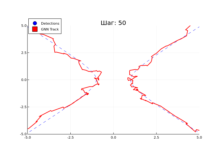
trackerGNN (generic function with 1 method)

The plot_tracks function visualizes the tracking process. The function creates a visualization that allows you to compare the operation of the algorithm with real values in dynamics, and includes the following logic.

Blue dots (scatter) – current measurements (detections).
The blue dotted lines represent the real trajectories of objects (obj1, obj2).
The red squares represent GNN tracks with a history (solid line).

function plot_tracks(tracks::Vector{Track}, detections::Vector{Detection}, obj1, obj2, step)
    p = scatter(getindex.(d.position[1] for d in detections), getindex.(d.position[2] for d in detections), label="Detections", color=:blue, markersize=6)
    # Real trajectories
    plot!(getindex.(p[1] for p in obj1[1:step]), getindex.(p[2] for p in obj1[1:step]), label="", color=:blue, linestyle=:dash)
    plot!(getindex.(p[1] for p in obj2[1:step]), getindex.(p[2] for p in obj2[1:step]), label="", color=:blue, linestyle=:dash)

    # Auxiliary function for rendering tracks
    function plot_tracks!(tracks, label, color, marker)
        for (i, t) in enumerate(tracks)
            scatter!([t.state[1]], [t.state[2]], label=i==1 ? label : "", color=color, markersize=8, marker=marker)
            # Rendering the track history
            if length(t.history) > 1
                plot!(getindex.(h[1] for h in t.history), getindex.(h[2] for h in t.history), 
                      label="", color=color, linestyle=:solid, linewidth=2)
            end
        end
    end
    
    # Tracks of different types with a history
    plot_tracks!(tracks, "GNN Track", :red, :square)
    plot!(legend=:topleft, title="Step: $step", xlims=(-5, 5), ylims=(-5, 5))
end

plot_tracks (generic function with 1 method)

The generate_hyperbola_trajections function generates two symmetric hyperbolic trajectories, namely, it creates a range of the parameter t from -3 to 3 with a uniform distribution, after which it calculates the coordinates of the points for two hyperbolas.

First: acosh(t), y = bsinh(t)
Second: -acosh(t), y = bsinh(t)

This feature is great for testing tracking algorithms on intersecting trajectories. It creates realistic test trajectories that simulate the movement of objects along hyperbolic paths.

# A function for generating hyperball trajectories
function generate_hyperbola_trajectories(steps, a=1.0, b=1.0)
    t = range(-3, 3, length=steps)
    [(a*cosh(ti), b*sinh(ti)) for ti in t], [(-a*cosh(ti), b*sinh(ti)) for ti in t]
end

generate_hyperbola_trajectories (generic function with 3 methods)

Now let's simulate and visualize hyperbolic trajectory tracking.

The simulation cycle includes the following steps.

An algorithm for adding Gaussian noise to real positions at each step.
Updates GNN trackers and visualizes the current status via plot_tracks.
Saves the last frame as a PNG image, and also creates an animated GIF (5 frames/seconds) of the entire tracking process.

steps = 50
obj1, obj2 = generate_hyperbola_trajectories(steps)

# Initializing tracks with a history
initial_state1 = [obj1[1][1], obj1[1][2], 0.5, 0.5]
initial_state2 = [obj2[1][1], obj2[1][2], -0.5, 0.5]
tracks_gnn = [Track(initial_state1, Matrix(1.0I, 4, 4), 1, 0),
              Track(initial_state2, Matrix(1.0I, 4, 4), 2, 0)]

# Creating a GIF
anim = @animate for step in 1:steps
    # Generating measurements for the current step
    noise = 0.3(randn(4))
    detections = [Detection([obj1[step][1] + noise[1], obj1[step][2] + noise[2]], step), 
                  Detection([obj2[step][1] + noise[3], obj2[step][2] + noise[4]], step)]
    # Updating the track
    updated_tracks_gnn = trackerGNN(detections, deepcopy(tracks_gnn), 50.0)
    # Updating the original tracks for the next step
    global tracks_gnn = updated_tracks_gnn
    # Visualization
    plot_tracks(tracks_gnn, detections, obj1, obj2, step)
    if step == steps
        savefig("last_frame.png")
    end
end 
# Saving the GIF
gif(anim, "tracking_simulation.gif", fps=5)

Conclusion

Results:

The last step of the simulation shows that the algorithm successfully tracks both objects, despite the added noise to the measurements.
The trajectories of the tracks (red lines) are close to the real trajectories of objects (blue dotted lines), which confirms the accuracy of the algorithm. At the same time, we see the biggest inaccuracies precisely at the moment when the trajectories touch.
The value LIIar: 50 – the threshold value for the Mahalonobis distance indicates the algorithm's resistance to false positives.

using Images
println("The last step of the simulation:")
img = load("last_frame.png")

Последний шаг моделирования:

The presented algorithm demonstrates high efficiency for tracking objects with nonlinear trajectories. The key advantages are:

noise resistance due to Kalman filter;
ease of implementation of the GNN method for comparing measurements;
Visual visualization that makes it easy to interpret the results.

The algorithm successfully solves the problem of tracking and can be applied in such areas as autonomous systems, video surveillance and robotics. To further improve the algorithm, we can consider using more complex motion models (for example, a constant acceleration model) or tracking methods such as JPDA or MHT to work in high-density environments.