Adjustment of the central frequency when exposed to interference
The example considers the construction of a radar with the possibility of adjusting the central frequency of the probing signal. This approach makes it possible to overcome the effects of active interference in the operating frequency band.
Functions used
function run_model( name_model, path_to_folder ) # defining a function for running the model
    Path = path_to_folder * "/" * name_model * ".engee"
    if name_model in [m.name for m in engee.get_all_models()] # Checking the condition for loading a model into the kernel
        model = engee.open( name_model ) # Open the model
        model_output = engee.run( model, verbose=true ); # Launch the model
        return nothing
        engee.close( name_model, force=true ); # Close the model
    else
        model = engee.load( Path, force=true ) # Upload a model
        model_output = engee.run( model, verbose=true ); # Launch the model
        engee.close( name_model, force=true ); # Close the model
    end
end

function WA2Data(X)
    out = collect(X)
    out_data = zeros(eltype(out.value[1]),size(out.value[1],1),size(out.value[1],2),length(out.value))
    [out_data[:,:,i] = out.value[i] for i in 1:length(out.value)]

    return out_data, out.time
end;
1. Description of the model
Unlike the example Monostatic radar with multiple целями in the current model, the following functional nodes have been updated and improved:
- pulse signal generator with linear frequency modulation, capable of tuning from one central frequency to another;
- Added interference effects in the operating frequency band
- Broadband channel usage
- Updating the signal processing algorithm
The radar operates at a frequency of 300 MHz with a sampling rate of 2 MHz. It is located at the origin point and is considered stationary. The target is about 10 km away and approaching at a speed of about 100 meters per second. The general block diagram is given below:
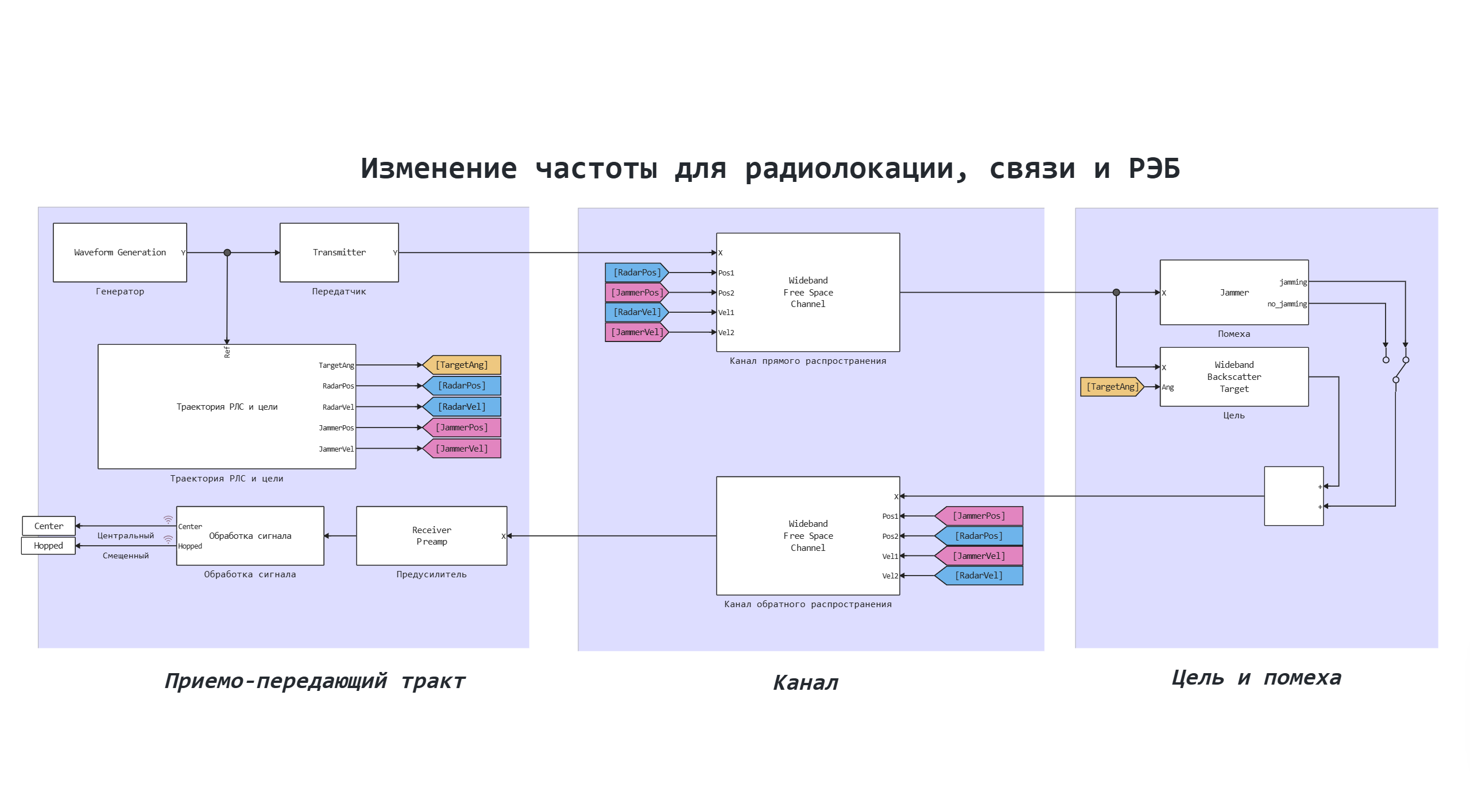
Let's take a closer look at the features of this model.:
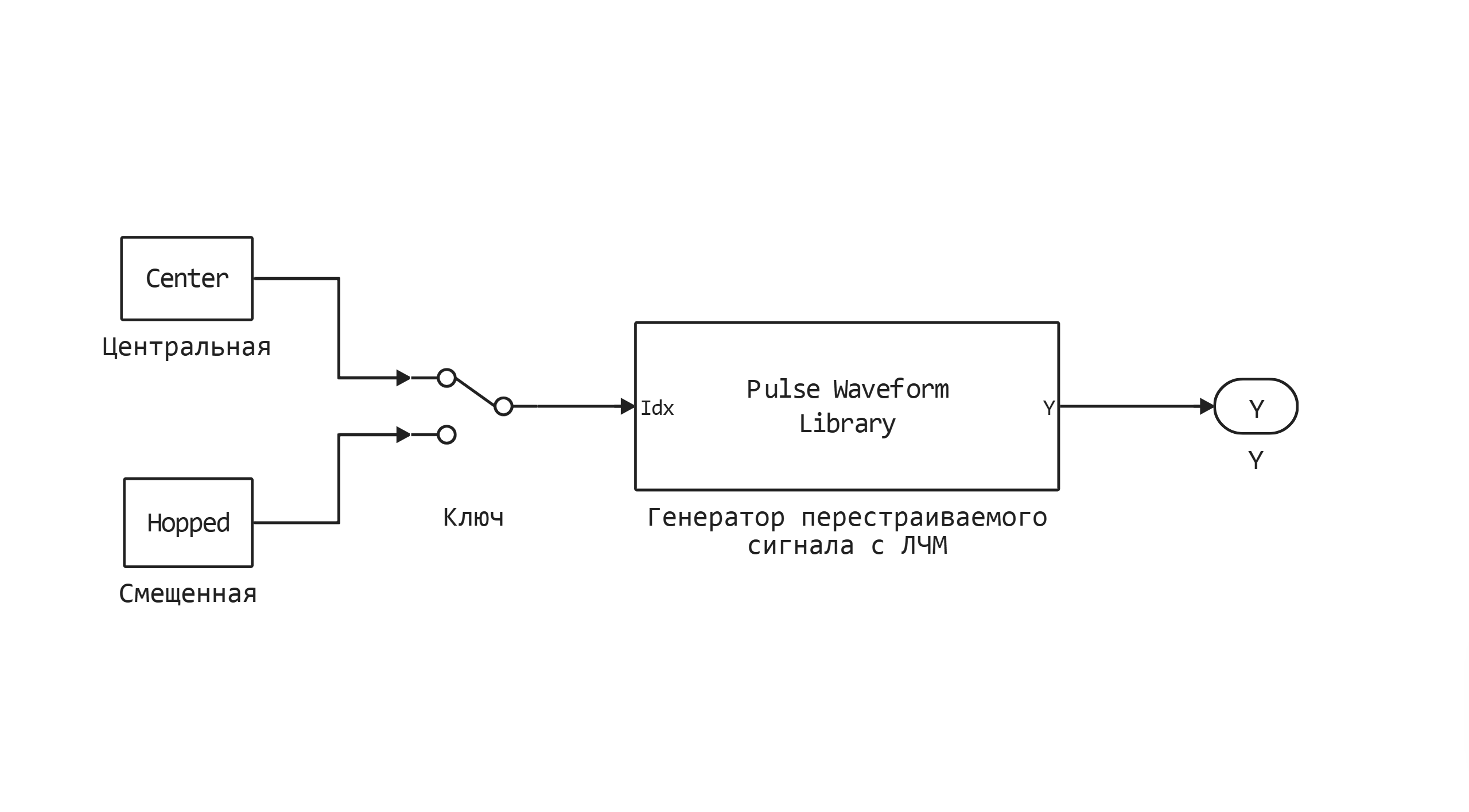
Generator (Waveform Generation)
The masked "Waveform Generation" block contains a tunable LF signal generator. Using the key, it is possible to switch between the center frequencies of 0 and 250 kHz.
Channel and Jammer </h4>
- Wideband Free Space: uses a broadband channel for direct and reverse distribution in free space;
- Jammer: A jamming model that simulates a useful signal at a false range
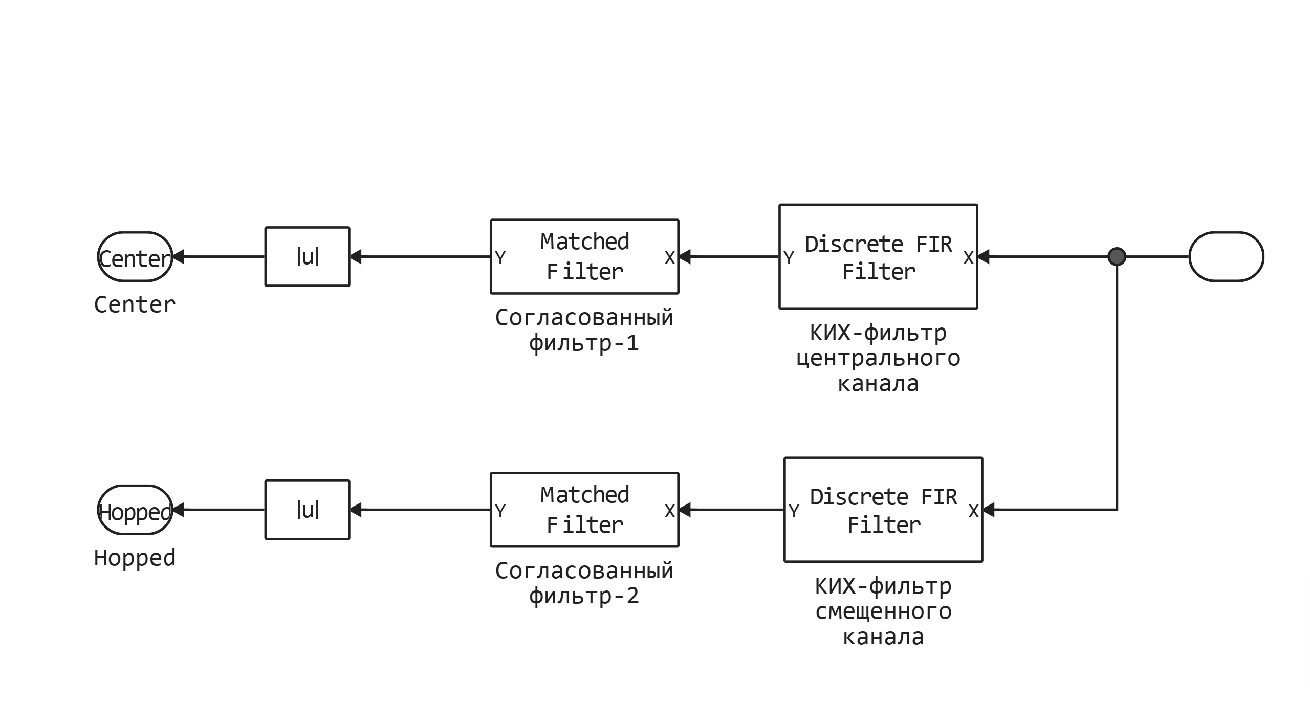
Signal Processing
After receiving the signal, it is necessary to select a useful signal for each band (in the example there are 2 of them) using a bandpass filter (Band Filter) tuned to the appropriate center band. After the signal is isolated, a matched filtering unit (Matched Filter) is used to increase the signal-to-noise ratio (SNR):
2. Initialization of input parameters
Connect the input parameter initialization file "FrequencyAgilityParam.jl"
include("$(@__DIR__)/FrequencyAgilityParam.jl");
The structure of the jl file is shown below:
fundamental parameters:
c = 3e8; # signal propagation speed
Fs = 2e6 # sampling rate

# Transmitter parameters
PeakPower = 5000 # Transmitter power, W
TxGain = 20 # Gain, dB
TxLossFactor = 0 # transmission path loss, dB
receiver parameters
NoisePower= 1e-12 # Noise power, W
RxGain = 20 # Receiver gain, dB
RxLossFactor = 0 # transmission path loss, dB
radar position and interference
JammerPos = [10_000 ;0;1_000] # initial interference position, m
JammerVel = [100;0;0] # interference velocity, m/s
RadarPos = [0 ;0;0] # radar initial position, m
RadarVel = [0 ;0;0] # radar velocity, m/s
If necessary, the file parameters can be changed, but it needs to be reconnected.
3. Launching the model
Using the model run function run_model, let's run a simulation of the model:
run_model("FrequencyAgility", @__DIR__); # launching the model
4. Reading simulation results
Using the function WA2Data counting the results from the Center and Hopped variables:
Center_engee,_ = WA2Data(Center) # central channel output
Hopped_engee,_ = WA2Data(Hopped); # offset channel output
5. Visualization of results
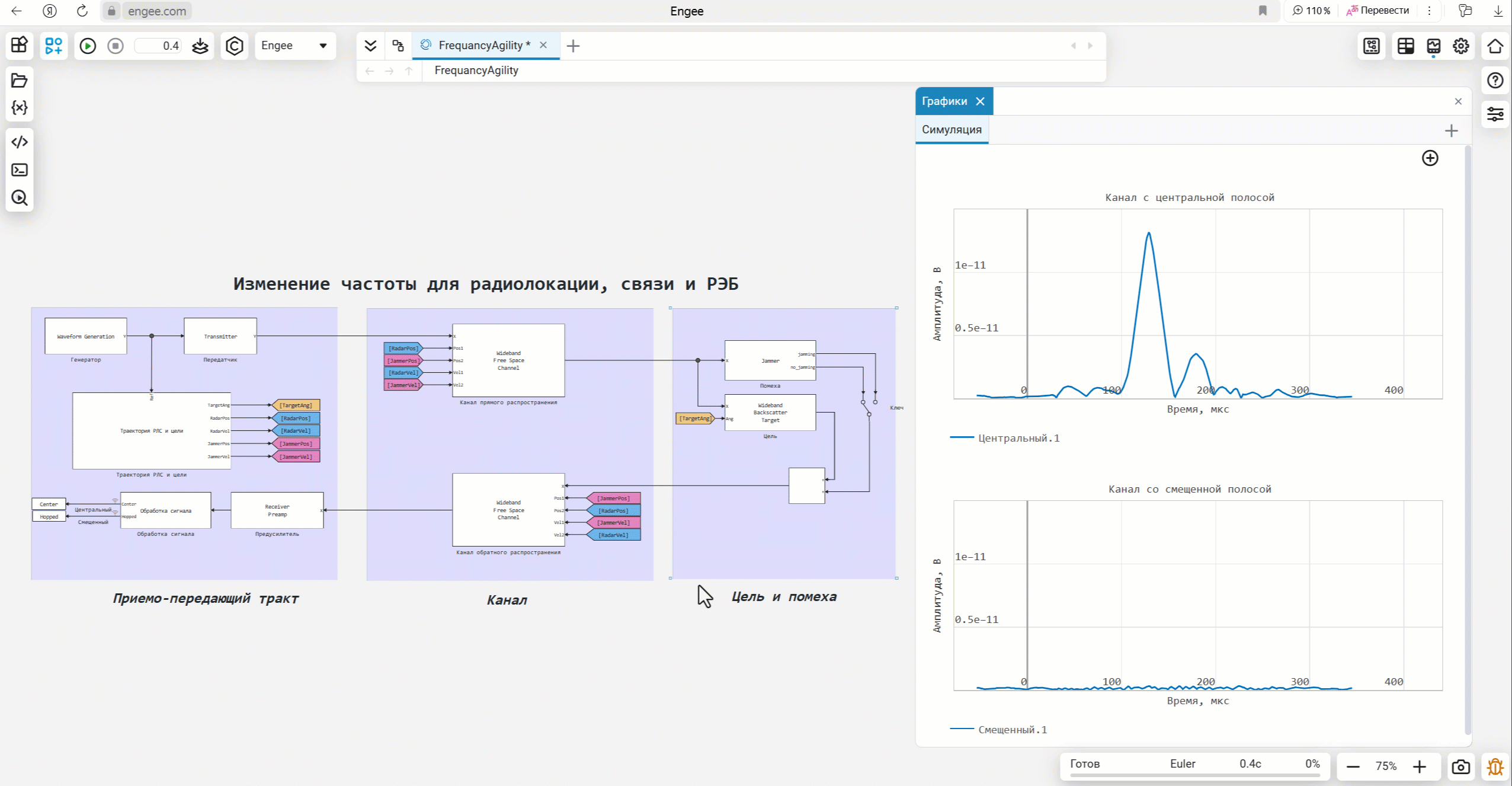
Let's plot the simulation results for the last pulse along the central and offset channels:
fig1 = plot(abs.(Center_engee[:,1,end]),label="The central channel",color="red",ylabel="The amplitude, In")
fig2 = plot(abs.(Hopped_engee[:,1,end]), label="Offset channel",xlabel="Time, counts",ylabel="The amplitude, In")
plot(fig1,fig2,layout=(2,1))
The central graph shows that the interference located at 185 counts suppresses the useful signal. In the shifted channel, only the receiver's own noise is present, since the useful and interfering signals are filtered out by the FIR filter.
6. Analysis of the model operation
Let's consider the radar operation scenario: suppose that at the initial moment of time a target is detected, after some time the interference effect is connected, and after that a frequency adjustment to an offset channel is implemented.
A visualization of the model's operation in the described mode is shown below (file **FrequencyAgility.gif **):
At the end of the recording, you can see that the frequency adjustment allowed you to "separate" the target and the active interference on different channels.
Conclusion
In the example, a method for dealing with active interference falling into the operating frequency band was considered. By adjusting the central frequency of the probing signal, it was possible to minimize the effect of interference on the operation of the radar system.