A system model of a single-position radar system with multiple targets

The model demonstrates the operation of a simple single-position radar system with multiple targets (4 by default), the coordinates of which are set in the ParamMMT.jl file.

In contrast to the example of modeling a monostatic radar with one целью in the receiving and transmitting path, it is possible to control the geometry of the antenna array, which forms a multi-lobed radiation pattern (DN).

1. Description of the model structure

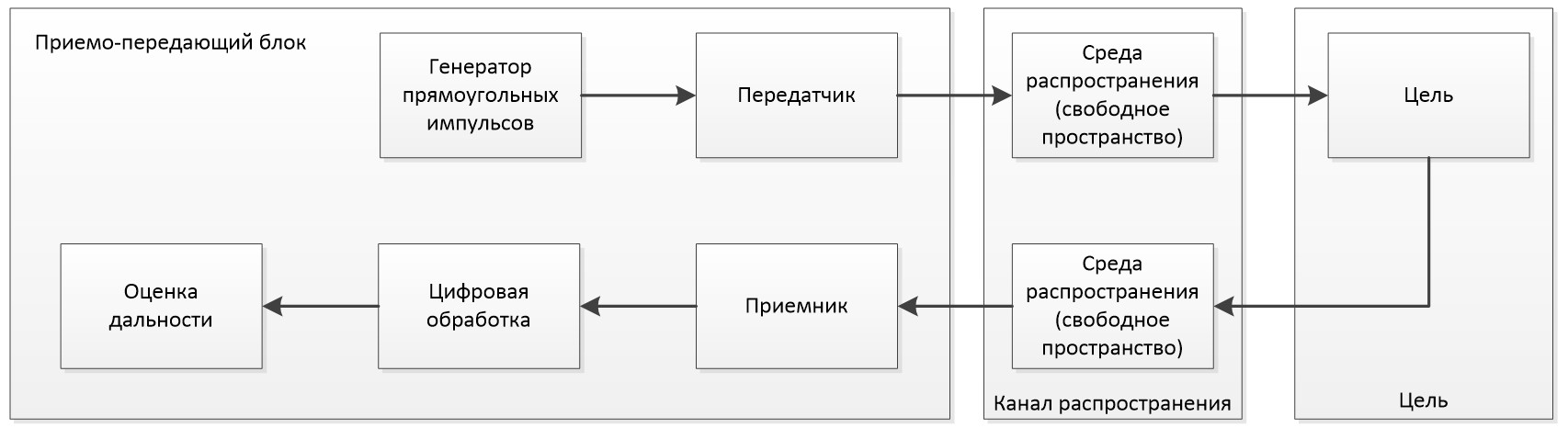
Let's take a closer look at the structural scheme of the model:

Source (Waveform Rectangular): A sequence of rectangular pulses is used as a probing signal;
Transmitter: The signal is amplified in the transmitter and the bottom is formed using an antenna array;
Distribution Environment (Free Space): The signal propagates to the targets and back to the receiver, undergoing attenuation proportional to the distance to the targets;
Target (Radar Target): Reflects the incoming signal and simulates the movement of both targets;
Receiver Preamp: The signal reflected from the targets arrives at the receiving antenna array and is amplified by adding the receiver's own thermal noise.
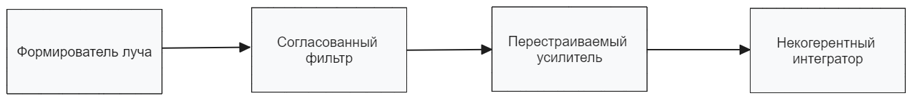
Digital Signal processing: Digital processing consists of the following steps: BeamFormer, Matched Felter, Tunable Gain, Incoherent accumulation (Pulse Integrator);

The model's operation scheme is shown in the figure below.

Digital processing consists of the following elements:

Based on the block diagram, we have developed the radar model shown in the figure below.

2. Initialization of input parameters

To initialize the input parameters of the model, we will connect the file "ParamMMT.jl". If you need to change the parameter values, then open this file and edit the necessary parameters.

include("$(@__DIR__)/ParamMMT.jl");
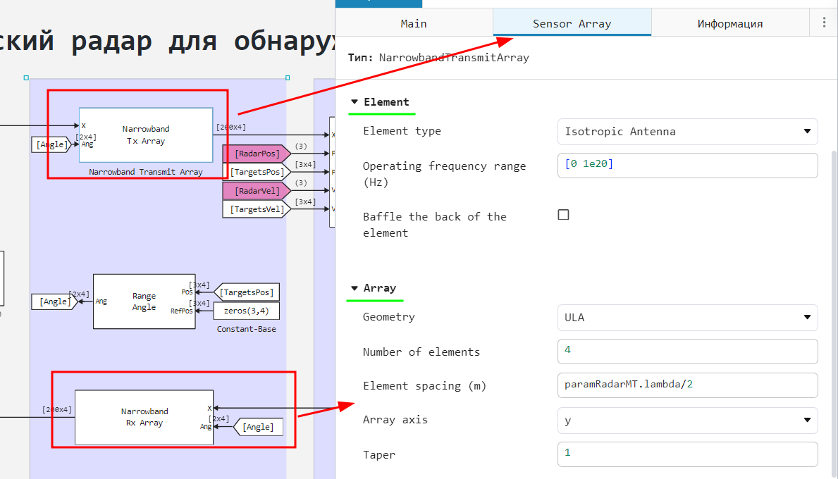
paramRadarMT = calcParams();

Flexible configuration of the antenna array of the transmitter and receiver is possible in the model, including: element type, antenna array geometry (an example of setting antenna array parameters is shown in the figure below):

Additionally, it is possible to visualize the ** radiation pattern** of the antenna array (AR) using the function pattern(). Let's build it based on the geometry from the picture above.:

# задание антенного элемента
antenna_element = EngeePhased.IsotropicAntennaElement(FrequencyRange=[0.0 1e20], BackBaffled=false)

# проектирование геометрии антенной решетки (в нашем случае ULA - линейная эквидистатная АР)
ULA_Array = EngeePhased.ULA(
    Element=antenna_element, # инициализация антенного элемента
    NumElements=4,# количество антенных элементов
    ElementSpacing=paramRadarMT.lambda/2, # расстояние между антенными элементами
    ArrayAxis="y", # ориентация элементов антенной решетки,
    Taper = 1 # весовой коэффициент антенного элемента
) 

# построение диаграммы направленности
pattern(ULA_Array,paramRadarMT.fc)

It can be seen from the bottom that along the y axis AR practically does not emit radiation, but it radiates best in the x-z plane.

3. Launching the model

function run_model( name_model, path_to_folder ) # определение функции для прогона модели
    Path = path_to_folder * "/" * name_model * ".engee"
    if name_model in [m.name for m in engee.get_all_models()] # Проверка условия загрузки модели в ядро
        model = engee.open( name_model ) # Открыть модель
        model_output = engee.run( model, verbose=true ); # Запустить модель
        engee.close( name_model, force=true ); # Закрыть модель
    else
        model = engee.load( Path, force=true ) # Загрузить модель
        model_output = engee.run( model, verbose=true ); # Запустить модель
        engee.close( name_model, force=true ); # Закрыть модель
    end
    return model_output
end;

out = run_model("MonostaticRadarMT", @__DIR__); # запуск модели

Building...
Progress 0%
Progress 7%
Progress 16%
Progress 27%
Progress 34%
Progress 42%
Progress 49%
Progress 55%
Progress 60%
Progress 65%
Progress 70%
Progress 76%
Progress 81%
Progress 88%
Progress 95%
Progress 100%
Progress 100%

4. Reading the output data

We calculate the necessary output from the out variable (in our case "out_MR_MT"):

result = (out["out_MR_MT"]).value;

5. Displaying the results

Let's build the system response at the last step of the model, obtained in the previous paragraph.:

out_step_end = result[end] # считывание последнего шага модели
R_engee = paramRadarMT.metersPerSample .* (0:size(out_step_end, 1) - 1) .+ paramRadarMT.rangeOffset # сетка дальности
# построение графика
plot(R_engee,abs.(out_step_end)*1e6,title="Сигнал на выходе модели после обработки от 4 целей",label="",
    xlabel="Расстояние,м",ylabel="Мощность приемника, мкВт",gridalpha=0.5,lw=2,color=:blue)

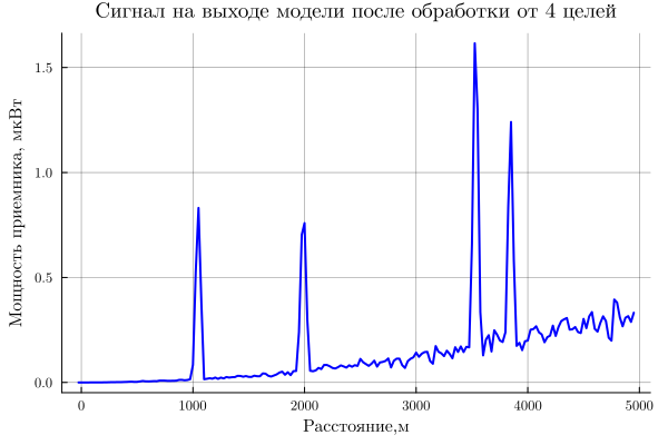
Conclusion

In the example, the operation of a simple single-position radar system was considered. As a result of the radar operation, 4 targets were detected at a previously set distance (1045, 1988, 3532 and 3845 meters).

Blocks used in example¶

Bitwise Operator