Car radar for estimating the range of a single target

The example considers the design of a system model of an automotive radar based on a linear frequency modulation (LFM) signal to determine the ranges of objects.

Functions used

Pkg.add(["LinearAlgebra", "DSP", "FileIO" ,"Images" , "ImageShow"])

using DSP,FFTW,LinearAlgebra

function run_model( name_model, path_to_folder ) # определение функции для прогона модели
    Path = path_to_folder * "/" * name_model * ".engee"
    if name_model in [m.name for m in engee.get_all_models()] # Проверка условия загрузки модели в ядро
        model = engee.open( name_model ) # Открыть модель
        engee.run( model, verbose=true ); # Запустить модель
        engee.close( name_model, force=true ); # Закрыть модель
    else
        model = engee.load( Path, force=true ) # Загрузить модель
        engee.run( model, verbose=true ); # Запустить модель
        engee.close( name_model, force=true ); # Закрыть модель
    end
    return
end;

function DataFrame2Array(X)
    out = collect(X)
    out_data = zeros(eltype(out.value[1]),size(out.value[1],1),size(out.value[1],2),length(out.value))
    [out_data[:,:,i] = out.value[i] for i in 1:length(out.value)]

    return out_data, out.time
end

function calc_spectrogram(x::Array,fs::Real,title::String;
    num_pulses::Int64 = 4,
    window_length::Int64 = 64,
    nfft::Int64=512,
    lap::Int64  = 60,
    thesh::Real = -Inf)

    gr()

    spec_out = DSP.spectrogram(x[:,:,1:num_pulses][:],window_length,lap;window=kaiser(window_length,3.95),nfft=nfft,fs=fs)

    power = DSP.pow2db.(spec_out.power)
    power .= map(x -> x < thesh ? thesh : x,power)

    power_new = zeros(size(power))

    power_new[1:round(Int64,size(power,1)/2),:] .= power[round(Int64,size(power,1)/2)+1:end,:]
    power_new[round(Int64,size(power,1)/2)+1:end,:] .= power[1:round(Int64,size(power,1)/2),:]

    fig = heatmap(fftshift(spec_out.freq).*1e-6,spec_out.time .*1e6, permutedims(power_new),color= :jet,
        gridalpha=0.5,margin=5Plots.mm,size=(900,400))
    xlabel!("Частота, МГц")
    ylabel!("Время, мкс")
    title!(title)

    return fig
end;

1. Description of the model structure

1.1 General scheme of the system model

The general block diagram of the system model is presented below:

Let's take a closer look at the model structure:

LFM Signal Generator (FMCW Waveform): A continuous LFM signal is used as a probe signal;
Transmitter: The signal is amplified in the transmitter and a radiation pattern is formed;
Propagation medium (Channel): the signal propagates to the targets and back to the receiver, while attenuation is taken into account depending on the distance to the target;
Object (Car): represents a moving car;
Receiver Preamp: The signal reflected from the machine enters the receiving antenna array and is amplified, taking into account the receiver's own thermal noise;
Digital Signal Processing: evaluates the range of a vehicle.

The model's operation scheme is shown in the figure below.

1.2 Description of the stages of digital signal processing

In the radar receiver, the reflected signal goes through several processing stages before an estimate of the range to the target object, the car, is obtained. The process of Signal Processing (Signal Processing) consists of two stages:

1st Stage: Range signal processing. The received signal is multiplied with the complex-conjugate input signal, resulting in a difference frequency (or beat frequency) due to the movement of the target between the reflected and the target area. Then there is a coherent accumulation of 64 pulses, which are combined in the subsystem Coherent Integration, which increases the signal-to-noise ratio. Next, the data is transmitted to the Range Response block, which performs a fast Fourier transform (FFT) for subsequent range estimation.
Stage 2: Object detection and range estimation consists of 5 parallel data processing channels for target object detection and range estimation.

In stage 2, each channel includes 3 processing steps:

Object detection: Radar data is first transmitted to a one-dimensional detector with a given probability of false alarms (CFAR) using a rolling-average window algorithm. This block detects the presence of a reflected signal.
Clustering: Then the clustering process is performed in the "DBSCAN Clusterer" block, where the detection cells are grouped into groups by range using the data obtained in the CFAR block.
Range estimation: in the final stage of defining detection objects and clusters, the last step is the Range Estimator block. At this stage, the target detection range is estimated based on radar data.

1.3 Channel model and goals

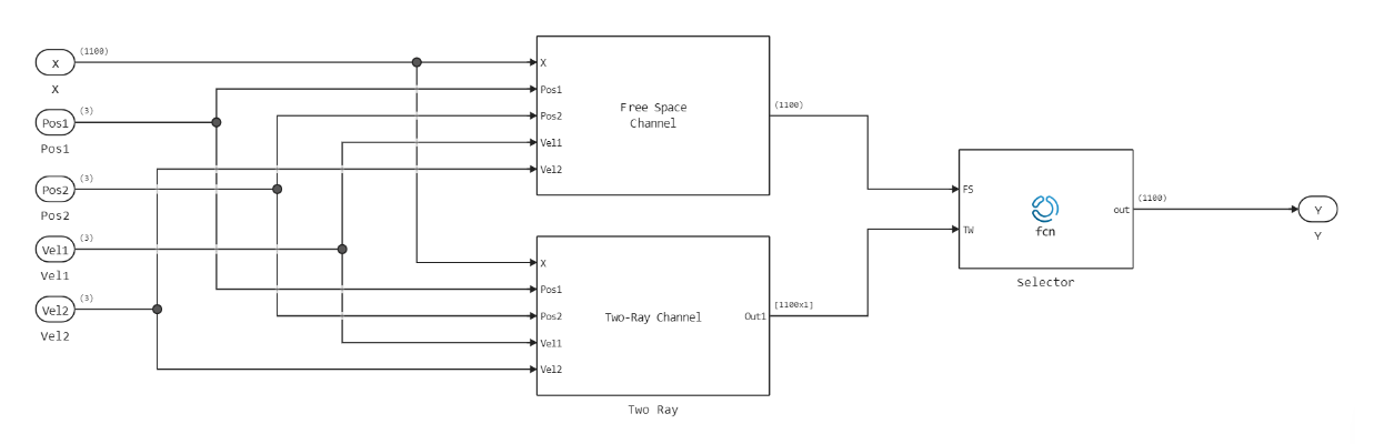
The subsystem of the "Channel and target" model simulates the propagation of a signal and its reflection from the target vehicle.

Channel — simulates the propagation of a signal between a radar vehicle and a target vehicle. The channel can be configured as a direct transmission channel in free space (model Free Space Channel) or as a two-beam channel in which the signal is transmitted to the receiver along both a direct and reflected path from the ground (model Two-Ray Channel). By default, a channel in free space is selected.

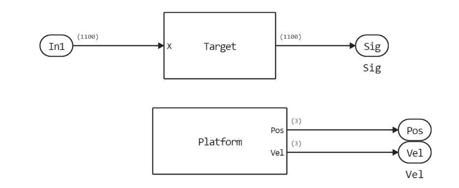
Target - Reflects the incident signal and simulates the trajectory of the target vehicle. The subsystem shown below consists of two parts: a target model to simulate a reflected signal (block - Target) and an object model in space to simulate the dynamics of the target vehicle (block - Platform).

2.Initialization of input parameters

In the model scenario, a vehicle equipped with radar starts moving from the reference point at a speed of 100 km/h (27.8 m/s), and the target object starts moving 43 meters in front of it at a speed of 96 km/h (26.7 m/s). The radar and target positions and speeds are used in the propagation channel to calculate the delay, Doppler effect, and signal attenuation.

To initialize the input parameters of the model, we will connect the file "FMCWParam.jl". If you need to change the parameter values, then open this file and edit the necessary parameters.

include("$(@__DIR__)/FMCWParam.jl") # подключение файла с входными параметрами
paramRadarFMCW = FMCWParam(); # запись входных параметров в структуру
T = paramRadarFMCW.T; # шаг дискретизации модели
simT = 640*T; # время симуляции модели

3. Launching the model

Let's start calculating the simulation of the model using the run_model function:

run_model("FMCW_Radar_Range_Estimation",@__DIR__); # Запустить модель

Building...
Progress 0%
Progress 0%
Progress 0%
Progress 5%
Progress 10%
Progress 15%
Progress 20%
Progress 25%
Progress 41%
Progress 46%
Progress 57%
Progress 63%
Progress 69%
Progress 83%
Progress 94%
Progress 100%

4. Reading the output data

We will extract the simulation results from the variables recorded in the workspace into an array for further visualization.:

input_signal, _ = DataFrame2Array(in_sig) # входной ЛЧМ-сигнал
dec_signal, _ = DataFrame2Array(dec_sig) # сигнал после цифровой обработки
range_estimate, slow_time = DataFrame2Array(rng_est) # оценки дальности
RPos, fast_time = DataFrame2Array(RPos) # положение радара
CPos,_ = DataFrame2Array(CPos); # положение объекта

5. Visualization of radar operation

5.1 Input signal spectrogram

First, let's consider the spectrogram of the emitted LFM signal.

calc_spectrogram(
    input_signal, # ЛЧМ-сигнал
    paramRadarFMCW.Fs, # частота дискретизации
    "Cпектрограмма ЛЧМ-сигнала";
    num_pulses=4 # количество импульсов отображения
)

The spectrogram shown above shows that the frequency deviation is 150 MHz with a period of every 7 microseconds, which corresponds to a resolution of about 1 meter.

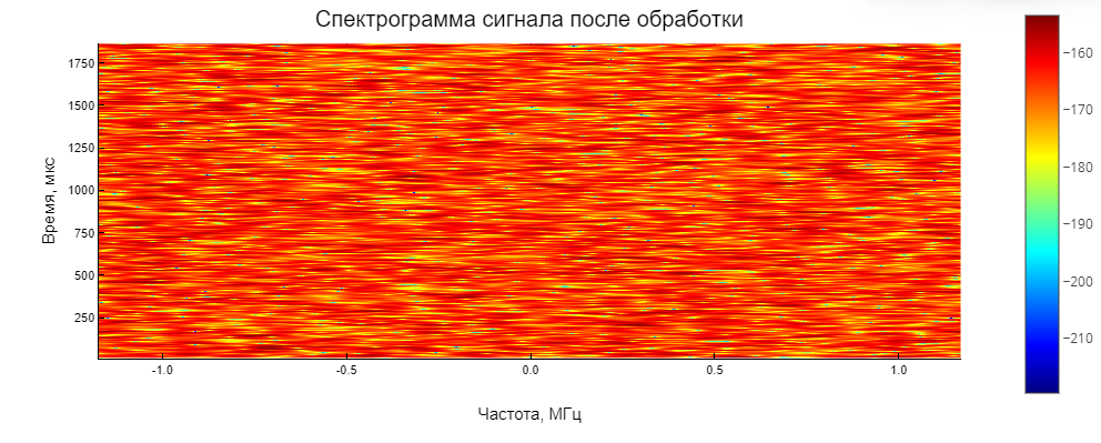
5.2 Signal spectrogram after digital processing

Next, consider the spectrogram of the signal after digital processing:

calc_spectrogram(
    dec_signal[:,:,2:end], # сигнал после обработки (отображается со 2 импульса)
    paramRadarFMCW.Fs/paramRadarFMCW.NumSweeps, # частота дискретизации
    "Cпектрограмма сигнала после обработки";
    num_pulses=4, # количество импульсов 
    thesh=-300 # порог, дБ
)

The graph shows that the beat frequency generated by the objects is approximately 100 kHz. Note that after processing, the signal has only one frequency component. The final range estimate is calculated based on the beat frequency, with an accuracy of 1 meter.

5.3 Estimating the distance to the object

And finally, let's look at the result of the radar operation.:

gr()
true_range = [norm(CPos[:,1,i].-RPos[:,1,i]) for i in 1:size(CPos,3)]
p1 = plot(Vector(slow_time)*1e3,range_estimate[:],label="оценка расстояния",margin=5Plots.mm,
    titlefont=font(10,"Computer Modern"),guidefont = font(8,"Computer Modern"),legendfont = font(8,"Computer Modern"))
plot!(Vector(fast_time)*1e3,true_range,label="истинное расстояние")
ylabel!("Расстояние, м")
title!("Зависимость оценки расстояния до цели от времени")

p2 = plot(Vector(slow_time)*1e3,abs.(range_estimate[:].-true_range[1:paramRadarFMCW.NumSweeps:end]),lab="",
titlefont=font(10,"Computer Modern"),guidefont = font(8,"Computer Modern"),legendfont = font(8,"Computer Modern"))
xlabel!("Время, мс")
ylabel!("Расстояние, м")
title!("Отклонение оценки")

plot(p1,p2,layout=(2,1),size=(900,460))

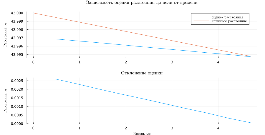
Thus, the accuracy of estimating the distance from the radar to the target object corresponds to the stated accuracy of 1 m.

5.4 Analysis of the effect of two-beam signal propagation

The result from the previous paragraph is achieved with the model of a direct propagation channel in free space. In fact, multiple paths between the transmitter and receiver are often used for transmission between vehicles. Therefore, signals from different paths can be combined either in phase or out of phase.

If we set up a two-ray propagation model ** (Two-Ray)**, which is the simplest multipath channel, we can see that the main beat frequency cannot be distinguished against the background of the noise spectrum (see the spectrogram below) because the direct signal is combined with the reflected one.

Filling up

In the example, the modeling of the basic model of an atomic radar with the use of a continuous LFM signal as a probing signal was considered. As a result of the model's operation, an estimate of the distance from the radar to the target object (car) was found with a radar resolution accuracy of 1 meter.

The influence of the signal propagation model was also investigated: the direct propagation channel and the bi-beam propagation channel. The results showed that the two-beam propagation model can negatively affect radar operation by compensating for the beat frequency component, and thereby making range estimation impossible.