Automotive radar for range and speed estimation of multiple targets¶

The example discusses the design of a system model of an automotive radar for estimating the range and speed of multiple targets.

Functions used¶

Pkg.add(["LinearAlgebra", "DSP"])

   Resolving package versions...
  No Changes to `~/.project/Project.toml`
  No Changes to `~/.project/Manifest.toml`

using DSP,FFTW,LinearAlgebra

function run_model( name_model, path_to_folder ) # определение функции для прогона модели
    Path = path_to_folder * "/" * name_model * ".engee"
    if name_model in [m.name for m in engee.get_all_models()] # Проверка условия загрузки модели в ядро
        model = engee.open( name_model ) # Открыть модель
        engee.run( model, verbose=true ); # Запустить модель
        engee.close( name_model, force=true ); # Закрыть модель
    else
        model = engee.load( Path, force=true ) # Загрузить модель
        engee.run( model, verbose=true ); # Запустить модель
        engee.close( name_model, force=true ); # Закрыть модель
    end
    return
end;

function DataFrame2Array(X)
    out = collect(X)
    out_data = zeros(eltype(out.value[1]),size(out.value[1],1),size(out.value[1],2),length(out.value))
    [out_data[:,:,i] = out.value[i] for i in 1:length(out.value)]

    return out_data, out.time
end

function calc_spectrogram(x::Array,fs::Real,title::String;
    num_pulses::Int64 = 4,
    window_length::Int64 = 64,
    nfft::Int64=512,
    lap::Int64  = 60,
    thesh::Real = -Inf)

    gr()

    spec_out = DSP.spectrogram(x[:,:,1:num_pulses][:],window_length,lap;window=kaiser(window_length,3.95),nfft=nfft,fs=fs)

    power = DSP.pow2db.(spec_out.power)
    power .= map(x -> x < thesh ? thesh : x,power)

    power_new = zeros(size(power))

    power_new[1:round(Int64,size(power,1)/2),:] .= power[round(Int64,size(power,1)/2)+1:end,:]
    power_new[round(Int64,size(power,1)/2)+1:end,:] .= power[1:round(Int64,size(power,1)/2),:]

    fig = heatmap(fftshift(spec_out.freq).*1e-6,spec_out.time .*1e6, permutedims(power_new),color= :jet,
        gridalpha=0.5,margin=5Plots.mm,size=(900,400))
    xlabel!("Частота, МГц")
    ylabel!("Время, мкс")
    title!(title)

    return fig
end

function calc_RD_Response(x,param;tresh=-Inf)
    plotlyjs()
    range_scale = Vector(range(param.RngLims...,length=size(x,1)))
    speed_scale = Vector(range(param.SpeedLims...,length=size(x,2)))

    out_RD = pow2db.(abs.(x[:,:,end]))
    out_RD  .= rot180(map(x -> x < tresh ? tresh : x,out_RD))

    fig = heatmap(speed_scale,range_scale,
        out_RD,colorscale=:parula256,
        top_margin=10Plots.mm,size=(900,400))
    xlabel!("Скорость, м/с")
    ylabel!("Дальность, м")
    title!("Дальностно-доплероский портрет")
    return fig
end

function plotting_result(rng_est,speed_est,true_range,true_speed,name::String,slow_time)
    plotlyjs()
    fig1=plot(slow_time*1e3,rng_est,
        lab="оценка расстояния",
        margin=5Plots.mm,
        legend=:outertopright,
        titlefont=font(12,"Computer Modern"),
        guidefont = font(12,"Computer Modern"),size=(900,220))
    plot!(fast_time*1e3,true_range,lab="истинное расстояние",ls= :dash)
    xlabel!("Время, мс")
    ylabel!("Расстояние, м")
    title!("Зависимость расстояния до объекта ($(name))")

    fig2 = plot(slow_time*1e3,speed_est,
        lab="оценка скорости",
        size=(900,220),
        legend=:outertopright,
        titlefont=font(12,"Computer Modern"),
        guidefont = font(12,"Computer Modern"))
    plot!(fast_time*1e3,true_speed,lab="истинная скорость",ls= :dash)
    xlabel!("Время, мс")
    ylabel!("Скорость, м/c")
    title!("Зависимость относительной скорости объекта ($name)")

    display(fig1)
    display(fig2)
    return
end

calc_range_or_speed_object(x,y) = [norm(x[:,1,i]).-norm(y[:,1,i]) for i in 1:size(y,3)];

WARNING: using LinearAlgebra.I in module Main conflicts with an existing identifier.

1. description of the system model structure¶

1.1 General structure of the model¶

The general structure diagram of the system model is given below:

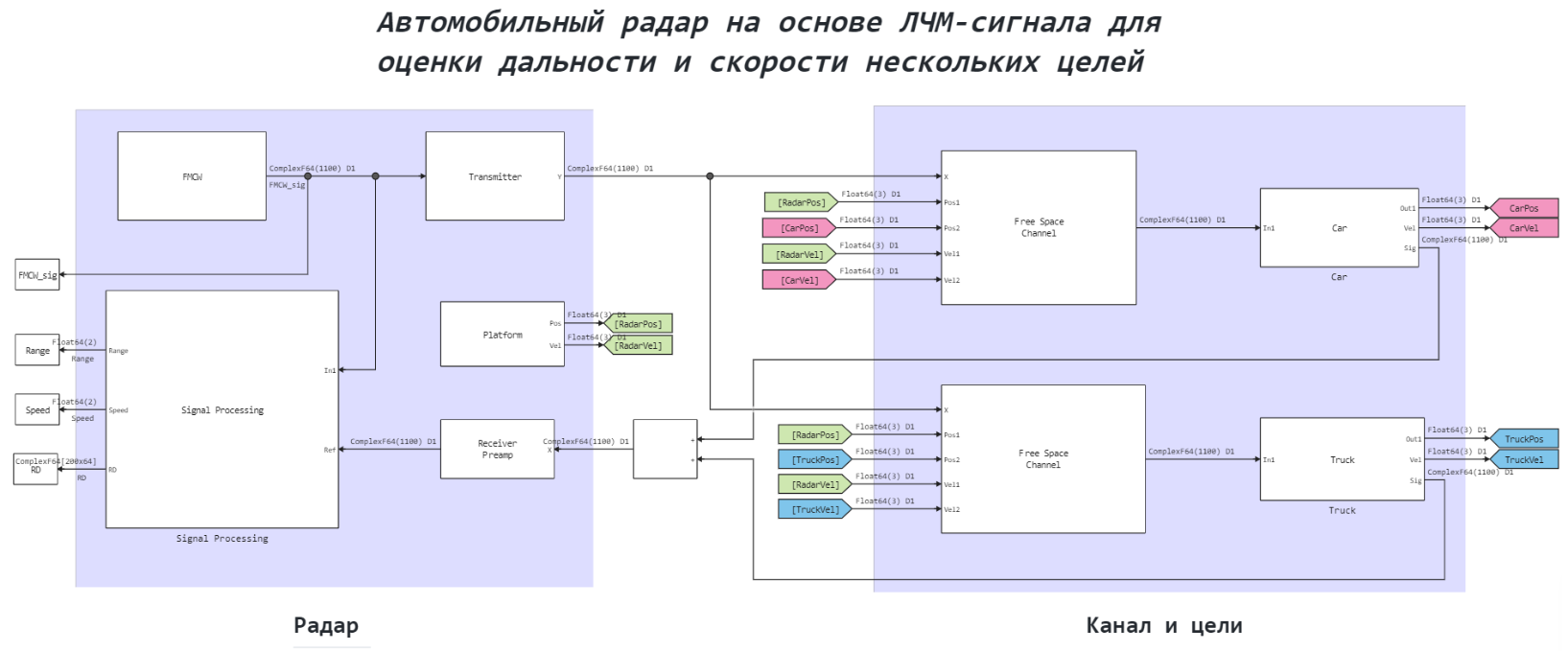
The model under consideration has a similar structure as in the example (single-target vehicle radar), but has a few key differences:

simulates the motion of 2 vehicles - a car and a lorry;
implements Doppler frequency processing using the "Range-Doppler Response " block;
single channel processing;
performs detection using a two-dimensional averaging detector using the "CA CFAR 2-D " block.

1.2 Digital Signal Processing Unit (Signal Processing)¶

The model uses combined range and Doppler frequency processing in the Signal Processing subsystem. This processing allows to estimate the frequency shift of the received signal relative to the probe signal during the coherent accumulation time, and then use the processing result for range and velocity estimation.

The digital signal processing subsystem is shown below:

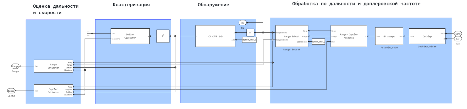
The digital processing process is divided into the following stages:

Stage 1: demodulation of the received signal and coherent accumulation of 64 pulses. Then the data is transferred to the Range-Doppler Response block to calculate the Range-Doppler Portrait of the received signal. The counts carrying range information are passed to the Range Subset subsystem. It extracts a part of the estimated data, which correspond to predefined range limits (from 1 to 200 m) in the calcParamFMCW.jl file;
Step 2: The detection process is carried out. The detector in this example is a CA CFAR 2-D unit that detects the signal;
Step 3: a clustering process is performed in the "DBSCAN Clusterer " block, which clusters the detection cells into range and velocity groups using the data obtained in the CA CFAR 2-D block;
Step 4: calculation of range and velocity estimates of targets using **Range Estimator* and **Doppler Estimator* blocks.

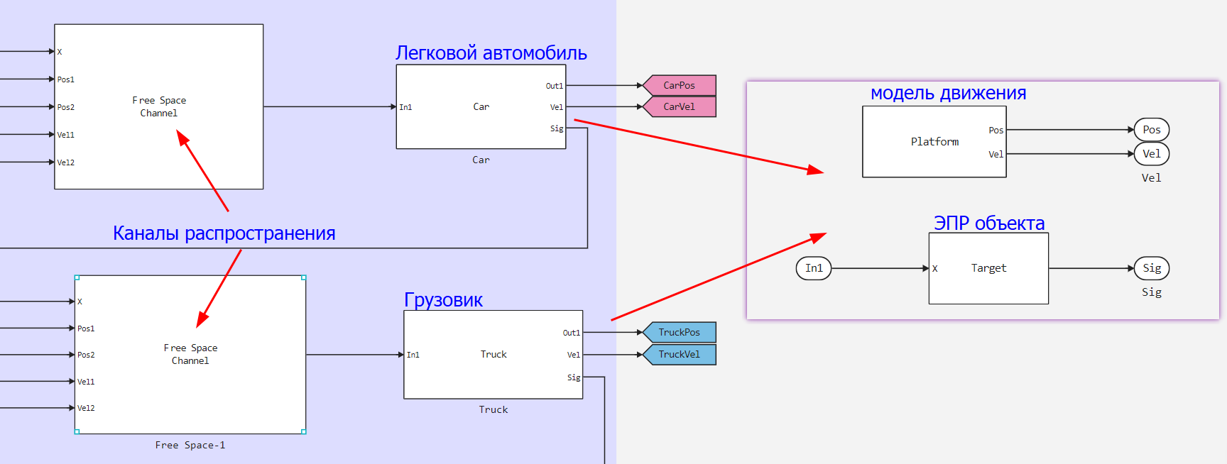
1.3 Channel and target models¶

The modelling scenario represents the following scenario: a vehicle with radar is moving from a reference point at 100 km/h (27.8 m/s)

There are two target vehicles present in the line of sight, which are a car and a lorry, each vehicle has a corresponding propagation channel. The car is 50 metres away from the radar and travelling at 60 km/h (16.7 m/s). The truck is 150 metres from the radar and is travelling at 130 km/h (36.1 m/s).

The signal propagation channel is free space.

2 Initialisation of input parameters¶

To initialise the input parameters of the model we connect the file "calcParamFMCWMT.jl". If you need to change the values of parameters, open this file and edit the necessary parameters.

include("$(@__DIR__)/calcParamFMCWMT.jl") # подключение jl файла для инициализации входных параметров
paramRadarFMCWMT = calcParamFMCWMT() # создание структуры входных параметров
T = paramRadarFMCWMT.T; # шаг дискретизации модели по времени
SimT = 10*paramRadarFMCWMT.NumSweeps*paramRadarFMCWMT.T; # время симуляции модели

3. Running the model¶

Let's run the model simulation calculation using the run_model function:

run_model("FMCW_Radar_Range_Estimation_MT",@__DIR__) # Запустить модель

Building...
Progress 0%
Progress 0%
Progress 0%
Progress 5%
Progress 10%
Progress 10%
Progress 15%
Progress 20%
Progress 25%
Progress 30%
Progress 36%
Progress 41%
Progress 50%
Progress 58%
Progress 70%
Progress 80%
Progress 100%

4. Extract the simulation results¶

Let's extract the simulation results from the variables recorded in the workspace into an array for further visualisation:

FMCW_signal, fast_time = DataFrame2Array(FMCW_sig) # входной ЛЧМ-сигнал
Range_Estimate, _ = DataFrame2Array(Range) # оценка дальности
Speed_Estimate, slow_time = DataFrame2Array(Speed) # оценки cкорости
RD_Response,_  = DataFrame2Array(RD); # дальностно-доплероский портрет
Truck_vel,_ = DataFrame2Array(Tvel) # скорость грузовика
Truck_pos,_ = DataFrame2Array(Tpos); # положение грузовика
Car_vel,_ = DataFrame2Array(Cvel) # скорость автомобиля
Car_pos,_ = DataFrame2Array(Cpos); # положение автомобиля
Radar_vel,_ = DataFrame2Array(Rvel) # скорость радара
Radar_pos,_ = DataFrame2Array(Rpos); # положение радара

5. Visualisation of simulation results¶

5.1 Spectrogram of the input signal¶

After completing the model run and reading the data into the array, we will visualise the spectrogram of the probing signal using the calc_spectrogram function:

calc_spectrogram(
    FMCW_signal, # сигнал после обработки (отображается со 2 импульса)
    paramRadarFMCWMT.Fs/paramRadarFMCWMT.NumSweeps, # частота дискретизации
    "Cпектрограмма входного сигнала";
    num_pulses=4, # количество импульсов 
    thesh=-300 # порог, дБ
)

The spectrogram above shows that the frequency deviation is 150 MHz with a period every 7 microseconds, which corresponds to a resolution of about 1 metre.

5.2 Range Doppler portrait¶

calc_RD_Response(RD_Response,paramRadarFMCWMT;tresh=-Inf)

In the figure, 2 targets at a distance of 50 and 150 metres can be noted. The velocity of the targets is difficult to accurately determine due to the low velocity resolution

5.3 Analysing the accuracy of parameter estimation¶

To better analyse the accuracy of the radar, we compare the true coordinates and velocities with the found estimates.

First, we calculate the true values of the parameters and extract the estimates into the corresponding variables:

# Расчет истинных дальностей и относительный скоростей до автомобиля
true_range_car = calc_range_or_speed_object(Car_pos,Radar_pos)
true_speed_car = calc_range_or_speed_object(Radar_vel,Car_vel)
# Расчет истинных дальностей и относительный скоростей до грузовика
true_range_truck = calc_range_or_speed_object(Truck_pos,Radar_pos)
true_speed_truck = calc_range_or_speed_object(Radar_vel,Truck_vel)
# Расчет оценок дальностей и относительный скоростей до автомобиля
Range_Estimate_Car = Range_Estimate[1,1,:]
Range_Estimate_Truck = Range_Estimate[2,1,:]
# Расчет оценок дальностей и относительный скоростей до грузовика
Speed_Estimate_Car = Speed_Estimate[1,1,:]
Speed_Estimate_Truck = Speed_Estimate[2,1,:];

Display the results in graphs for each object using the plotting_result function:

 # графики для сравнения объекта - автомобиль
 plotting_result(Range_Estimate_Car,Speed_Estimate_Car,true_range_car,true_speed_car,"автомобиль",slow_time)

 # графики для сравнения объекта - грузовки
plotting_result(Range_Estimate_Truck,Speed_Estimate_Truck,true_range_truck,true_speed_truck,"грузовик",slow_time)

Analysing the obtained dependencies, we can conclude that the values of radar estimates correspond to the declared accuracy in terms of range (1 metre) and speed (4 m/s)

Conclusion¶

In the example we have considered the modelling of a basic model of an automotive radar using a continuous LFM signal as a probing signal. As a result of the model work, an estimate of the onositive speed and distance from the radar to the objects (car and truck) was found with a radar resolution accuracy of 1 metre for range and approximately 4 m/s for speed.