Detection Curves (ROC) Part 2: Monte Carlo simulation

This example shows how to build a receiver detection curve (ROC curve) of a radar system using Monte Carlo simulation. The ROC determines how well the system can detect targets, while discarding large false alarm values when the target is missing (false alarms). The detection system determines the presence or absence of a target by comparing the received signal value with a set threshold.

Probability of correct detection (Pd) is the probability that the instantaneous value of the signal is greater than the threshold value when the target is actually present.

False Alarm Probability (Pfa) is the probability that the signal value is greater than the threshold when the target is missing. In this case, the signal is caused by noise, and its properties depend on noise statistics. Monte Carlo simulation generates a very large number of radar signals in the presence and absence of a target.

The ROC curve is a graph of the dependence of Pd on Pfa. The shape of the ROC curve depends on the signal-to-noise ratio (SNR) of the received signal. If the SNR of the received signal is known, then the ROC curve shows how reliable the system is by analyzing the values of Pd and Pfa. If you set Pd and Pfa, you can determine what power is needed to meet this requirement.

You can use the rocsnr function to calculate theoretical ROC curves. This example shows the ROC curve obtained as a result of Monte Carlo simulation of a single antenna radar system, and compares this curve with the theoretical curve.

Tactical and technical characteristics of the radar

Set the desired Pd = 0.9 and Pfa = , we will set the maximum radar range of 4000 meters and a range resolution of 50 meters. Set the actual target range to 3,000 meters. We will also set the effective scattering area (ESR) of the target to 1.5 and an operating frequency of 10 GHz.

Pkg.add(["DSP"])
using DSP

   Resolving package versions...
  No Changes to `~/.project/Project.toml`
  No Changes to `~/.project/Manifest.toml`

using DSP

c = 299_792_458; # скорость распространения сигнала в пространстве, м/с
pd = 0.9; # вероятность правильного обнаружения
pfa = 1e-6; # вероятность ложной тревоги
max_range = 4000; # максимальная дальность, м
target_range = 3000.0; # дальность до цели, м
range_res = 50; # разрешение по дальности,м
tgt_rcs = 1.5; # ЭПР цели, м^2
fc = 10e9; # несущая частота, Гц
lambda = c/fc; # длина волны, м

Any simulation that calculates Pfa and pd requires processing multiple signals. In order not to take up a lot of memory, we will process only parts of the pulses. We will set the number of pulses to process 45_000 and the size of each part 10_000.

Npulse = 45_000; # количество импульсов
Npulsebuffsize = 10_000; # количество отсчетов в импульсе

Selection of the type of probing signal and its parameters

Let's create a system object for the LFM signal generator. To do this, you need to calculate:

Pulse band using range resolution;
Pulse repetition rate (PPI), based on the maximum range of the radar.
Sampling rate (fs) set the bandwidth to double, since the signal is broadband;
Pulse duration, based on the bandwidth.

pulse_bw = c/(2*range_res); # полоса импульса
prf = c/(2*max_range); # частота следования импульсов
fs = 2*pulse_bw; # частота дискретизации
pulse_duration = 10/pulse_bw; # длительность импульса

# Формирование генератора ЛЧМ-сигнала
waveform = EngeePhased.LinearFMWaveform(
    PulseWidth=pulse_duration,
    SampleRate=fs,
    SweepBandwidth=pulse_bw,
    PRF=prf
);

To achieve certain Pd and Pfas, it is required that sufficient signal power is supplied to the receiver after the target reflects the signal. Let's calculate the minimum SNR value required to achieve a given false alarm probability and detection probability using the Albersham equation.

snr_min = albersheim(pd,pfa); # минимальное значение ОСШ
println("ОСШ = $(round(snr_min;sigdigits=4)) дБ")

ОСШ = 13.11 дБ

To achieve SNR = 13 dB, sufficient power must be transmitted to the target. Use the radar equation to estimate the peak transmission power required to achieve a given SNR for a target at a range of 3,000 meters. The received signal also depends on the EPR, which is assumed to correspond to the non-fluctuating model (Swerling 0). We will set the radar to have the same gain coefficients for reception and transmission, equal to 20 dB.

txrx_gain = 20; # усиление передатчика и приемника

# Расчет дальности с помощью основного уравнения радилокации
peak_power = ((4*pi)^3*noisepow(1/pulse_duration)*target_range^4*
    DSP.db2pow(snr_min))/(DSP.db2pow(2*txrx_gain)*tgt_rcs*lambda^2) # 
println("peak_power = $(round(peak_power;sigdigits=5)) Вт")

peak_power = 293.18 Вт

Setting the parameters of the system objects of the transmitter

Let's create system objects that define the transmitting part of the simulation: the antenna motion model, antenna geometry, transmitter and radiator.

# модель движения радара
antennaplatform = EngeePhased.Platform(
    InitialPosition=[0; 0; 0], # начальное положение радара
    Velocity=[0; 0; 0] # компоненты вектора скорости радара
); 
# антенный элемент
antenna = EngeePhased.IsotropicAntennaElement(
    FrequencyRange=[5e9 15e9] # диапазон частот
);
# передатчик
transmitter = EngeePhased.Transmitter(
    Gain=txrx_gain, # усиление
    PeakPower=peak_power, # пиковая мощность
    InUseOutputPort=true # состояние радара
);
radiator = EngeePhased.Radiator(
    Sensor=antenna, # антенный элемент
    OperatingFrequency=fc # несущая частота
);

Setting up a Goal object

Create a Target object corresponding to a real reflective target with the specified EPR. Reflections from this target will simulate real reflected signals. To calculate false alarms, create a second target with zero EPR. Reflections from this target are zero, except for noise.

target = [EngeePhased.RadarTarget() EngeePhased.RadarTarget()] # вектор целей
targetplatform = [ EngeePhased.Platform()  EngeePhased.Platform()] # вектор моделей движения целей
# задание параметров целей
target[1] = EngeePhased.RadarTarget(
    MeanRCS=tgt_rcs, # ЭПР 
    OperatingFrequency=fc # несущая частота
);
target[2] = EngeePhased.RadarTarget(
    MeanRCS=1e-16,
    OperatingFrequency=fc
)
# задание параметров движения целей
targetplatform[1] = EngeePhased.Platform(
    InitialPosition=[target_range; 0; 0] # начальное положение
)

targetplatform[2] = EngeePhased.Platform(
    InitialPosition=[target_range; 0; 0] # начальное положение
);

Setting the parameters of a distribution environment object

Let's set the conditions for signal propagation - the propagation channels from the radar to the targets and back.

channel = [EngeePhased.FreeSpace() EngeePhased.FreeSpace()]
channel[1] = EngeePhased.FreeSpace(
    SampleRate=fs, # частота дискретизации
    TwoWayPropagation=true, # модель двунаправленного распространения
    OperatingFrequency=fc # несущая частота
);
channel[2] = EngeePhased.FreeSpace(
    SampleRate=fs, # частота дискретизации
    TwoWayPropagation=true,  # модель двунаправленного распространения
    OperatingFrequency=fc # несущая частота
);

Setting the parameters of the system object of the transmitter

Let's generate noise by setting the NoiseMethod property to "Noise temperature", and the noise temperature property to ReferenceTemperature to 290 K.

# Геометрия приемной антенны
collector = EngeePhased.Collector(
    Sensor=antenna, # антенна
    OperatingFrequency=fc # Несущая частота
);
# формирование передатчика
receiver = EngeePhased.ReceiverPreamp(
    Gain=txrx_gain, # усиление
    NoiseMethod="Noise temperature", # источник шумов - тепловые шумы
    ReferenceTemperature=290.0, # шумовая температура
    NoiseFigure=0, # фактор шума
    SampleRate=fs, # частота дискретизации
    EnableInputPort=true # синхронизация с передатчиком
);
# Задание начального значения источника шума
receiver.SeedSource = "Property";
receiver.Seed = 2010;

Setting the Fast Time grid

A fast time grid is a set of time samples within the pulse duration. Each count corresponds to a range resolution element.

fast_time_grid = unigrid(0,1/fs,1/prf,"[)"); # сетка быстрого времени
rangebins = c*fast_time_grid/2; # элементы разрешения по дальности

Generation of a probing signal

We will generate the pulses of the probing signal that you want to transmit.

wavfrm = waveform(); # формирования ЛЧМ-сигнала

Next, we will create a transmitted signal that includes the amplification of the transmitted antenna.

sigtrans,tx_status = transmitter(wavfrm);

Create consistent filter coefficients from the waveform object. Then create a consistent filter system object.

MFCoeff = getMatchedFilter(waveform); # коэффициенты фильтра
matchingdelay = size(MFCoeff,1) - 1; # заддержка на согласованную фильтрацию
mfilter = EngeePhased.MatchedFilter( # согласованный фильтр
    Coefficients=MFCoeff,
    GainOutputPort=false 
);

Calculating the range to the target

Calculate the range to the target, and then calculate the element number in the range resolution vector. Since the target and radar are stationary, the position and velocity values are used throughout the simulation cycle. It can be assumed that the number in the resolution vector is constant throughout the simulation.

# параметры движения радара и целей
ant_pos = antennaplatform.InitialPosition;
ant_vel = antennaplatform.Velocity;
tgt_pos = targetplatform[1].InitialPosition;
tgt_vel = targetplatform[1].Velocity;
# Расчет дальности и азимутальный угол от радара до целей
tgt_rng,tgt_ang = rangeangle(tgt_pos,ant_pos);
# поиск номера элемента разрешения по дальности
rangeidx = val2ind(tgt_rng,rangebins[2]-rangebins[1],rangebins[1])[1];

Pulse overlap

Let's create a signal processing cycle. Each step is performed by executing system objects. The processing cycle is called twice: once for the "target is present" condition and once for the "target is missing" condition.

Radiating a signal into space using EngeePhased.Radiator.
Signal propagation to the target and back to the antenna using EngeePhased.FreeSpace
Reflection of the signal from the target using EngeePhased.Target.
Passing the received signal through the reception amplifier using EngeePhased.ReceiverPreamp.This step also adds random noise to the signal.
Receiving the reflected signal to the antenna using EngeePhased.Collector.
Matched amplified signal filter using EngeePhased.MatchedFilter.
Save the output of the matched filter in the bin index of the target range for further analysis.

rcv_pulses = zeros(ComplexF64,length(sigtrans),Npulsebuffsize);
h1 = zeros(ComplexF64,Npulse,1);
h0 = zeros(ComplexF64,Npulse,1);
Nbuff = floor(Int64,Npulse/Npulsebuffsize);
Nrem = Npulse - Nbuff*Npulsebuffsize;
for n = 1:2 # H1 and H0 Hypothesis
    trsig = radiator(sigtrans,tgt_ang);
    trsig = channel[n](trsig,
        ant_pos,tgt_pos,
        ant_vel,tgt_vel);
    global trsig  = trsig
    rcvsig = target[n](trsig);
    rcvsig = collector(rcvsig,tgt_ang);
    
    for k = 1:Nbuff
        for m = 1:Npulsebuffsize
            rcv_pulses[:,m] = receiver(rcvsig, .!(tx_status.>0));
        end
        rcv_pulses = mfilter(rcv_pulses);
        rcv_pulses = buffer(rcv_pulses[(matchingdelay+1):end][:,:],size(rcv_pulses,1));
        if n == 1
            h1[(1:Npulsebuffsize) .+ (k-1)*Npulsebuffsize] = transpose(rcv_pulses[rangeidx,:]);
        else
            h0[(1:Npulsebuffsize) .+ (k-1)*Npulsebuffsize] = transpose(rcv_pulses[rangeidx,:]);
        end
    end
    if (Nrem > 0)
        for m = 1:Nrem
            rcv_pulses[:,m] = receiver(rcvsig, .!(tx_status.>0));
        end
        rcv_pulses = mfilter(rcv_pulses);
        rcv_pulses = buffer(rcv_pulses[(matchingdelay+1):end][:,:],size(rcv_pulses,1));
         if n == 1
            h1[(1:Nrem) .+ Nbuff*Npulsebuffsize] = transpose(rcv_pulses[rangeidx,1:Nrem]);
        else
            h0[(1:Nrem) .+ Nbuff*Npulsebuffsize] = transpose(rcv_pulses[rangeidx,1:Nrem]);
         end
    end
end;

Plotting histograms of outputs of matched filters

Let's calculate the histograms of the "target present" and "target absent" signals. Use 100 samples to get a rough estimate of the spread of the signal values. Let's set the limits of the histogram values from the smallest signal to the largest.

h1a = abs.(h1);
h0a = abs.(h0);
thresh_low = minimum([h1a;h0a]);
thresh_hi  = maximum([h1a;h0a]);
nbins = 100;
binedges = range(thresh_low,thresh_hi;length=nbins);
histogram(h0a,label="Target Absent",)
histogram!(h1a,label="Target Present")
title!("Target-Absent Vs Target-Present Histograms")

Comparison of simulated and theoretical Pd and Pfas

To calculate Pd and Pfa, count the number of cases when the "target is missing" return and the "target is present" return exceed the specified threshold. This set of thresholds has a finer granularity than the bins used to create the histogram in the previous simulation. Then we normalize these counts by the number of pulses to get a probability estimate. The sim_pfa vector is the modeled probability of a false alarm as a function of the threshold. The sim_pd vector is the modeled probability of detection, which is also a function of the threshold. The receiver sets the threshold so that it can determine the presence or absence of a target. The histogram above shows that the best threshold is about 1.8.

nbins = 1000;
thresh_steps = range(thresh_low,thresh_hi;length=nbins)
sim_pd = zeros(1,nbins)
sim_pfa = zeros(1,nbins)
for k = 1:nbins
    thresh = thresh_steps[k]
    sim_pd[k] = sum(h1a .>= thresh)
    sim_pfa[k] = sum(h0a .>= thresh)
end
sim_pd = sim_pd./Npulse;
sim_pfa = sim_pfa./Npulse;

To construct an experimental ROC curve, it is necessary to invert the Pfa curve so that a Pd vs Pfa graph can be plotted. You can invert the Pfa curve only if you can express the Pfa as a strictly monotonically decreasing function of the Threshold. To express the Pfa in this way, find all the indexes of the array for which the Pfa is a constant in neighboring indexes. Then delete these values from the Pd and Pfa arrays.

pfa_diff = diff(sim_pfa[:])
idx = (pfa_diff.!=0).*(1:length(pfa_diff))
sim_pfa = sim_pfa[idx[idx .!= 0]]
sim_pd = sim_pd[idx[idx .!= 0]];

Let's limit the smallest value of Pfa to .

minpfa = 1e-6;
N = sum(sim_pfa .>= minpfa)
sim_pfa = reverse(sim_pfa[1:N])
sim_pd = reverse(sim_pd[1:N]);

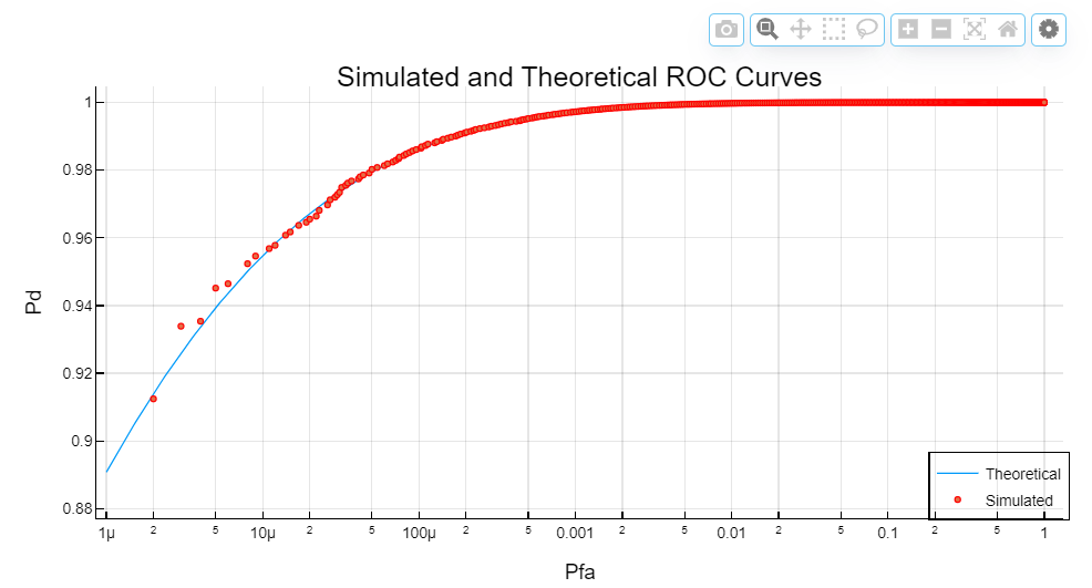
Calculate the theoretical values of Pfa and Pd from the lowest Pfa to 1. Then plot the theoretical Pfa curve.

theor_pd,theor_pfa = rocsnr(snr_min,"Pd&Pfa",
    SignalType="NonfluctuatingNoncoherent",
    MinPfa=minpfa,NumPoints=N,NumPulses=1);
plot(theor_pfa,theor_pd,label="Theoretical",legend_position=:bottomright,
    legend_background_color =:transparent)
scatter!(sim_pfa,sim_pd,lab = "Simulated",xscale= :log10,ms=2,
    markerstrokecolor = :red)
title!("Simulated and Theoretical ROC Curves")
xlabel!("Pfa")
ylabel!("Pd")

Improved simulation with one million pulses

In the previous simulation, Pd values with low Pfa do not fall along a smooth curve and do not even reach the set operating mode. The reason for this is that at very low Pfa levels, very few, if any, samples exceed the threshold. To generate curves with low Pfa, it is necessary to use the number of samples of the inverse Pfa order. This type of modeling takes a lot of time. The following curve uses a million pulses instead of 45,000. To run this simulation, repeat the example, but set Npulse to 1000000.