Adaptive beamforming when exposed to interference

This example demonstrates the application of adaptive beamforming algorithms MVDR and LCMV under conditions of two interfering signals.

Auxiliary functions

# запуск симуляцик системной модели
function run_model( name_model, path_to_folder ) # определение функции для прогона модели
    Path = path_to_folder * "/" * name_model * ".engee"
    if name_model in [m.name for m in engee.get_all_models()] # Проверка условия загрузки модели в ядро
        model = engee.open( name_model ) # Открыть модель
        model_output = engee.run( model, verbose=true ); # Запустить модель
        engee.close( name_model, force=true ); # Закрыть модель
    else
        model = engee.load( Path, force=true ) # Загрузить модель
        model_output = engee.run( model, verbose=true ); # Запустить модель
        engee.close( name_model, force=true ); # Закрыть модель
    end
    return model_output
end;

# считывание выходных данных
function calc_array_out(out, name)
    array = zeros(eltype(out[name].value[1]),size(out[name].value[1],1),size(out[name].value[2],2),length(out[name].value))
    [array[:,:,i] = collect(out[name].value[i]) for i in eachindex(out[name].value)]
    return array
end

# построение выходных графиков
default(titlefontsize=11,top_margin=-1Plots.mm,guidefont=10,
   fontfamily = "Computer Modern",colorbar_titlefontsize=8,bottom_margin = -6Plots.mm
)

function plot_result(out, title, number, t_step = 0.3)
    t = Vector(0:t_step/size(out, 1):t_step*(1-1/size(out, 1)))*1e3 # сетка времени в мс
    plot(t, out[:, 1, number], label = title, title = title,size=(500,150))
    plot!(t, out_ref_pulse[:, 1, number], label = "Эталонный сигнал", 
        xlabel = "Время (мс)", уlabel = "Амплитуда (В)"
    )
end;

1. Description of the model structure

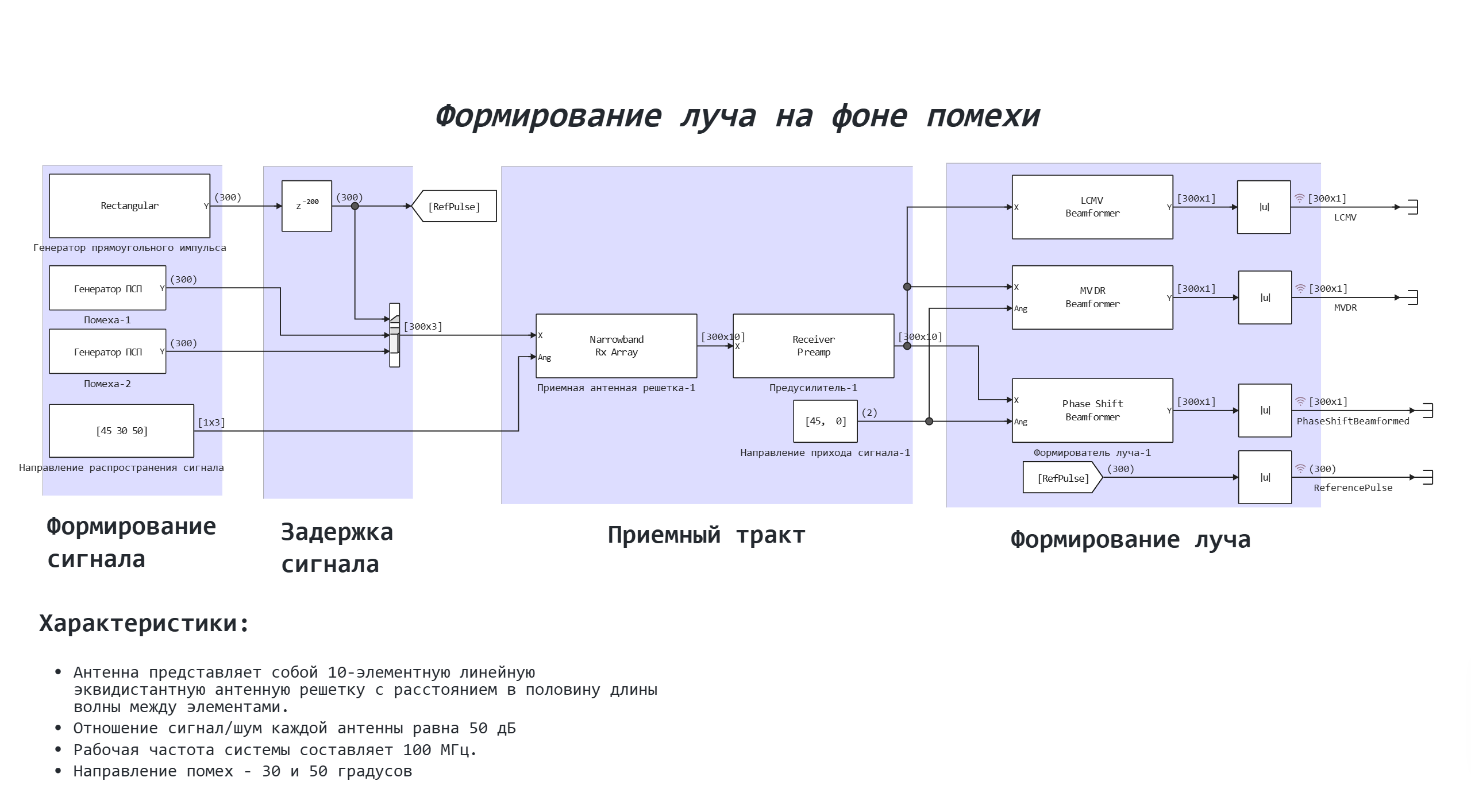
The model illustrates the formation of a beam in the presence of two interfering signals coming from azimuthal angles of 30 and 50 degrees. The amplitudes of the interfering signals are much larger than the amplitude of the pulse. The noise level is set to -50 dBW to emphasize only the effect of interference. The PhaseShift, MVDR, and LCMV beamforming algorithms are applied to the received signal, and their results are compared.

The structural diagram of the model is based on the example of the [classical beamforming] model (https://engee.com/community/ru/catalogs/projects/formirovanie-lucha-na-fone-shuma ) with the addition of new blocks:

PSP generator - simulates an interference component having a normal distribution law
Propagation direction - sets the direction of reception of the useful signal and interference signals in the block Receiving antenna array
MVDR shaper - implements the MVDR shaping algorithm in a given direction;
- LCMV Shaper - implements the LCMV shaping algorithm with a given weight matrix in a given direction;

The block diagram of the system is shown below.

2. Initialization of model parameters

The model parameters are set in the file ParamBeamformarI.jl using the auxiliary function calcParamBeamformerI. This function is performed once when the model is loaded. It exports a structure to the workspace, the fields of which are referenced by the dialog panels of the model. To change any parameters, either change the values in the structure from the command line, or edit the auxiliary function and restart it to update the parameter structure.

Model Parameters

# Radar parameters
propSpeed = physconst("LightSpeed") # Propagation velocity (m/s)

fc = 100e6 # Carrier frequency (Hz)
lambda = propSpeed/fc # Wavelength (m)

# Antenna Array parameters
numElements = 10 # number of items
ElementSpacing = 0.5*lambda # distance between elements (m)

Antenna = EngeePhased.ULA(numElements=10,ElementSpacing=0.5*lambda)

# Parameters of the probing signal
fs = 1000; # sampling rate of 1 kHz
prf = 1/0.3; # pulse repetition rate (Hz)

# Receiving device
NoisePower = 1/db2pow(50); # Noise Power (W)

Gain = 0.0 # Gain (dB))
LossFactor = 0.0 # Receiver Loss (dB)

# Matrix of weights for LCMV beam shaper
steeringvec = EngeePhased.SteeringVector(SensorArray=Antenna)
cMatrix = steeringvec(fc,[43 45 47])

# подключение файла с параметрами модели
include("$(@__DIR__)/ParamBeamformerI.jl");

3. Launching the model

Using the function run_model let's run a simulation of the system model Beamformer_Interference. We will write the generated simulation results into a variable out.

out = run_model("Beamformer_Interference", @__DIR__) # запуск модели

Building...
Progress 0%
Progress 10%
Progress 20%
Progress 60%
Progress 100%
Progress 100%

SimulationResult(
    "PhaseShift" => WorkspaceArray{Matrix{Float64}}("Beamformer_Interference/PhaseShift")
,
    "LCMV" => WorkspaceArray{Matrix{Float64}}("Beamformer_Interference/LCMV")
,
    "MVDR" => WorkspaceArray{Matrix{Float64}}("Beamformer_Interference/MVDR")
,
    "ReferencePulse" => WorkspaceArray{Vector{Float64}}("Beamformer_Interference/ReferencePulse")

)

4. Reading the output data

Using the function calc_array_out counting data from a variable out for each pledged output.

out_ref_pulse = calc_array_out(out, "ReferencePulse") # Эталонный импульс
out_lcmv = calc_array_out(out, "LCMV") # Формиватель луча LCMV
out_mvdr = calc_array_out(out, "MVDR") # Формиватель луча MVDR
out_phase_shift = calc_array_out(out, "PhaseShift"); # Формиватель луча PhaseShift

5. Visualization of the results of the model

Visualization of the results is possible in two ways:

in the "graphs" tab (by selecting the "array construction" graph type)
in a script using the data obtained as a result of the simulation

Using the first method, we visualize the result of the model for outputs with and without ray shaping.:

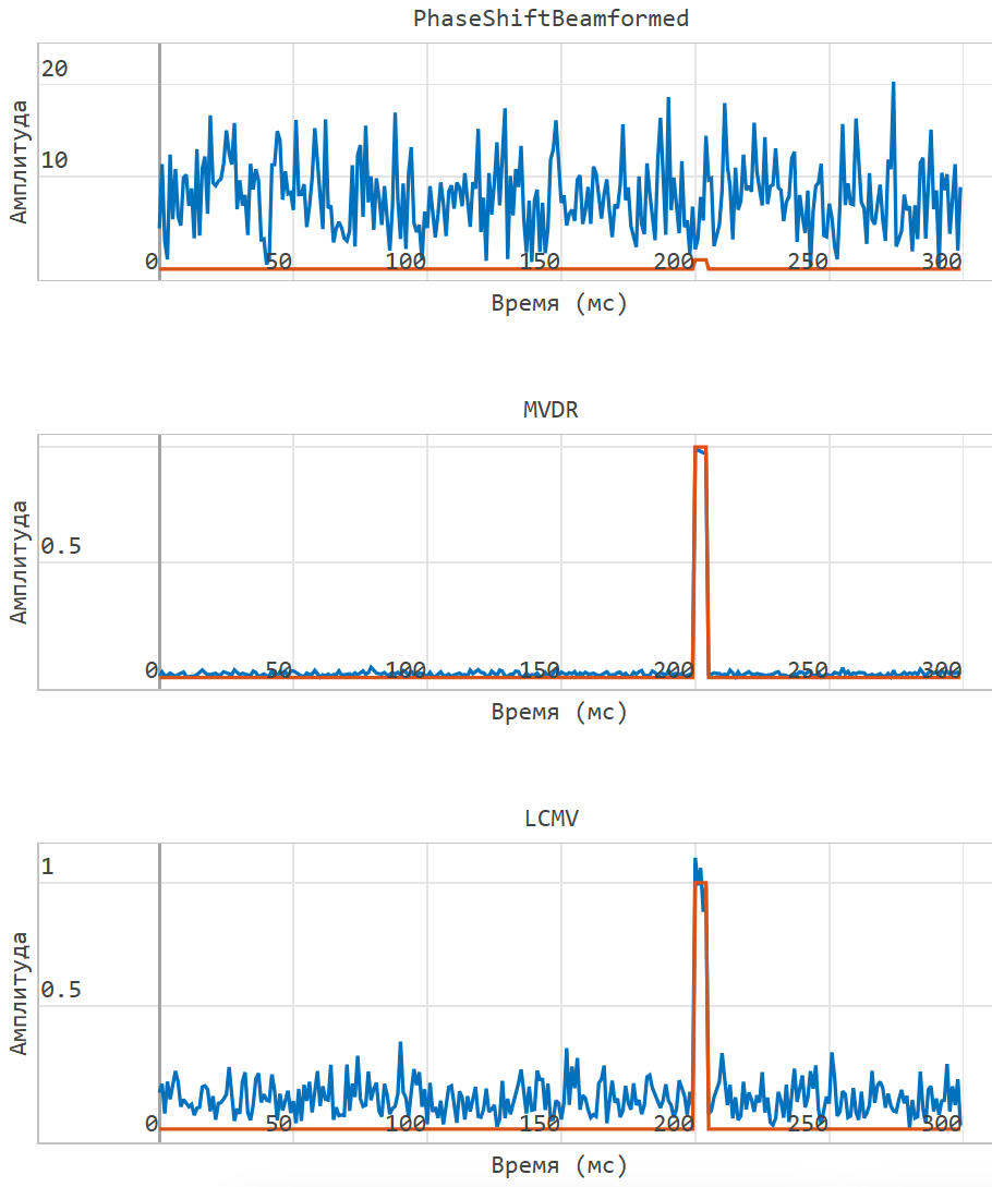
The figures show the output of 3 preset beam shapers: PhaseShift, MVDR and LCMV. It can be noted that the classical phase shift beamformer does not cope with the task of detecting a target against a background of interference because the interference amplitude is much larger than the useful signal and simply increasing the signal-to-noise ratio is not enough.

The output graph changes if the MVDR and LCMV beamforming algorithm is used: after signal processing, a peak corresponding to the true position of the target is formed.

Similarly, you can visualize the simulation results using the second method. To build it in the script, use the auxiliary function plot_result:

num_puls = length(collect(out["ReferencePulse"]).time) # извлечение номера последнего импульса
plot_result(out_phase_shift, "Формиватель PhaseShift", num_puls, t_step) |> display
plot_result(out_mvdr, "Формиватель MVDR", num_puls, t_step) |> display
plot_result(out_lcmv, "Формиватель LCMV", num_puls, t_step)

Comparing the resulting graphs, you can see that the resulting images are identical.

Conclusion

In the example, a comparison was made between simple and adaptive beam shapers against the background of a strong interference component. The results showed that the conventional phase shift shaper "PhaseShift Beamformer" is not able to detect a useful signal, in such cases it is necessary to resort to more advanced shaping algorithms "MVDR" or "LCMV"

Blocks used in example¶

Vector Concatenate