Multi-position Frequency Modulated (MFSK) car radar
The example examines the design of an automotive radar based on a multi-position frequency modulation (MFSK) signal to estimate the range and speed of several objects.
Functions used
Pkg.add(["LinearAlgebra", "DSP"])
include("$(@__DIR__)/calcParamMFSK.jl")

using DSP,FFTW,LinearAlgebra

function run_model( name_model, path_to_folder ) # defining a function for running the model
    Path = path_to_folder * "/" * name_model * ".engee"
    if name_model in [m.name for m in engee.get_all_models()] # Checking the condition for loading a model into the kernel
        model = engee.open( name_model ) # Open the model
        engee.run( model, verbose=true ); # Launch the model
        engee.close( name_model, force=true ); # Close the model
    else
        model = engee.load( Path, force=true ) # Upload a model
        engee.run( model, verbose=true ); # Launch the model
        engee.close( name_model, force=true ); # Close the model
    end
    return
end;

function DataFrame2Array(X)
    out = collect(X)
    out_data = zeros(eltype(out.value[1]),size(out.value[1],1),size(out.value[1],2),length(out.value))
    [out_data[:,:,i] = out.value[i] for i in 1:length(out.value)]

    return out_data, out.time
end

function calc_spectrogram(x::Array,fs::Real,title::String;
    num_pulses::Int64 = 4,
    window_length::Int64 = 32,
    nfft::Int64=32,
    lap::Int64  = 30,
    thesh::Real = -Inf)

    gr()

    spec_out = DSP.spectrogram(x[:,:,1:num_pulses][:],window_length,lap;window=kaiser(window_length,3.95),nfft=nfft,fs=fs)

    power = DSP.pow2db.(spec_out.power)
    power .= map(x -> x < thesh ? thesh : x,power)

    power_new = zeros(size(power))

    power_new[1:round(Int64,size(power,1)/2),:] .= power[round(Int64,size(power,1)/2)+1:end,:]
    power_new[round(Int64,size(power,1)/2)+1:end,:] .= power[1:round(Int64,size(power,1)/2),:]

    fig = heatmap(fftshift(spec_out.freq).*1e-6,spec_out.time .*1e3, permutedims(power_new),color= :jet,
        gridalpha=0.5,margin=5Plots.mm,size=(900,400))
    xlabel!("Frequency, MHz")
    ylabel!("Time, ms")
    title!(title)

    return fig
end;
1. Description of the model structure
The block diagram is similar to the example (Automotive radar for estimating the range and speed of multiple targets). The main differences are:
- Using a continuous radiation generator with multi-position frequency modulation;
- Signal processing that takes into account two parameters: the beat frequency and the phase shift between scans
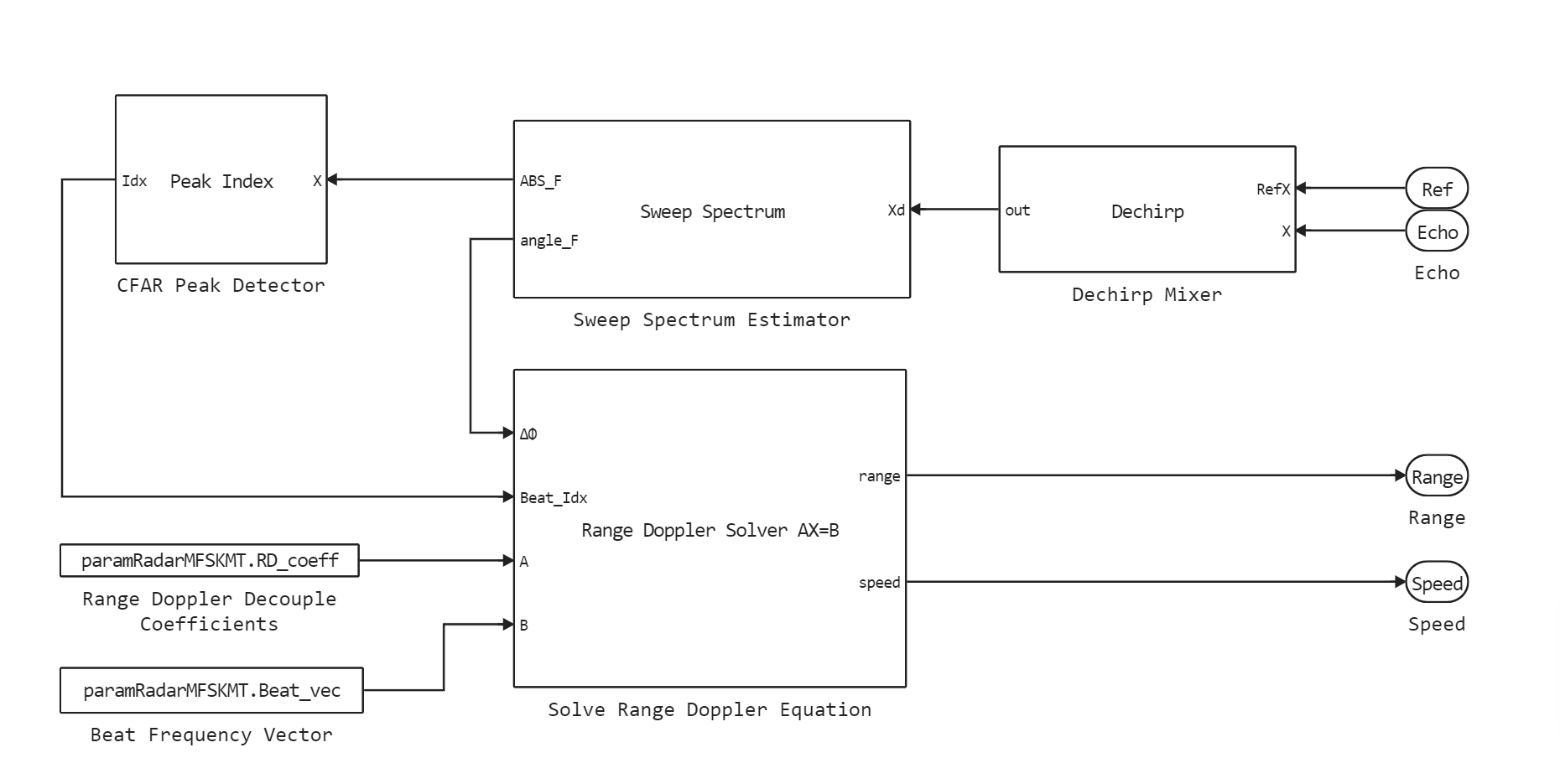
Signal processing unit
.png)
The signal processing subsystem consists of the following stages:
- The received signal is multiplied with the complex conjugate input signal in the Dechirp block, as a result of which the signal is demodulated;
- At the next stage, the demodulated signal is processed in the Sweep Spectrum block, where its spectrum in the frequency domain is calculated using the fast Fourier transform;
- Next, the process of detecting peaks in the spectrum corresponding to the targets takes place using a one-dimensional detector (CA CFAR Detector)
- At the final stage, using the found values of the beat frequencies and the phase difference between the sweeps, estimates of the range and speed of targets are calculated in the Solve Range Doppler Equation block.;
2. Initialization of input parameters
The simulation scenario is the following scenario: a vehicle with radar is moving from a reference point at a speed of 100 km/h (27.8 m/s)
There are ** two target vehicles** in the viewing area, which are a passenger car and a truck, each vehicle has a corresponding distribution channel. The car is moving at a distance of 50 meters from the radar and is moving at a speed of 60 km/h (16.7 m/s). The truck is located at a distance of 150 meters from the radar and is moving at a speed of 130 km/h (36.1 m/s).
The signal propagation channel is a free space.
To initialize the input parameters of the model, we will connect the file "calcParamMFSK.jl". If you need to change the parameter values, then open this file and edit the necessary parameters.
include("$(@__DIR__)/calcParamMFSK.jl") # connecting a file with validation parameters
paramRadarMFSKMT = CalcParamMFSK(); # validation of input parameters
T = paramRadarMFSKMT.T; # The modeling step
SimT = T; # Simulation time
3. Launching the model
run_model("MFSK_Radar_Range_Estimation_MT",@__DIR__); # Launching the model
4. Reading simulation results
sig_MFSK, fast_time = DataFrame2Array(MFSK) # the LCHM input signal
out_range, _ = DataFrame2Array(Range) # the signal after digital processing
out_speed, slow_time = DataFrame2Array(Speed); # range estimates
5. Visualization of radar operation
5.1 Input signal spectrogram
Let's construct a spectrogram of the input signal using the calc_spectrogram function
calc_spectrogram(
    sig_MFSK, # The LFM signal
    paramRadarMFSKMT.Fs, # sampling rate
    "Signal spectrogram with MFSK";
    num_pulses=1 # number of display pulses
)
The frequency component of the LC spectrogram has a stepwise character, which corresponds to a multi-position frequency modulation of the signal. In fact, the MFSK signal consists of two FMCW signal scans with a fixed discrete frequency offset. The scanning time of the emitted signal, which is determined by the product of a discrete step by the number of steps, is approximately 2 ms, which is several orders of magnitude longer than for a continuous LFM signal (about 7 microseconds).
5.2 Estimating the range and speed of objects
Let's analyze the result of the radar operation
Let's compare estimates and true values of ranges and speeds (the range to a car is 50 m, to a truck is 150 m)
println("Car range estimate $(round(out_range[1,1,end];sigdigits=5)) m")
println("Truck range estimate $(round(out_range[2,1,end];sigdigits=5)) m")

println("Car range estimate $(round(out_range[1,1,end]-50;sigdigits=5)) m")
println("Truck range estimate $(round(out_range[2.1,end]-150;sigdigits=5)) m")
Now let's compare the estimates and the true speed values (the relative speed of a car is 40 km/h, a truck is -30 km/h)
println("Estimation of the relative speed of the car $(round(out_speed[1,1,end]*3.6;sigdigits=5)) km/h")
println("Estimation of the relative speed of the truck $(round(out_speed[2.1,end]*3.6;sigdigits=5)) km/h")
println("The error in estimating the relative speed of the car is $(round(out_speed[1,1,end]*3.6-40;sigdigits=5)) km/h")
println("The error in estimating the relative speed of the truck is $(round(out_speed[2.1,end]*3.6-(-30);sigdigits=5)) km/h")
Analyzing the simulation results obtained, it can be concluded that the values of the radar estimates correspond to the stated accuracy in range (1 meter) and speed (1 km/h)
Conclusion
In the example, the design of an atomic radar model using a probe signal with multi-position frequency modulation was considered. As a result of the model, an estimate of the relative speed and distance from the radar to objects (car and truck) was found with a radar resolution accuracy of 1 meter in range and approximately 1 km/h in speed.
It should also be noted that the use of the considered signal made it possible to increase the scanning time compared to a continuous FM signal from 7 microseconds to 2 ms, which can reduce the cost of equipment.