Multi-sample signal detection

This example shows how to detect a signal in complex white Gaussian noise using multiple received signal samples. A matched filter is used to take advantage of the processing.

Introduction

The example "Detecting a signal against a background of white noise" presents a basic signal detection problem. Only one sample of the received signal is used for detection. In this example, more samples are used in the detection process to increase the detection efficiency.

As in the previous example, assume the signal strength is 1 and the signal-to-noise ratio (SNR) of one sample is 3 dB. The number of Monte Carlo trials is 100,000. The desired false alarm probability level (Pfa) is 0.001.

Ntrial = Int64(1e5); # количество испытаний Монте-Карло 
Pfa = 1e-3; 
snrdb = 3; # SNR в дБ 
snr = db2pow(snrdb); # SNR в линейном масштабе 
npower = 1/snr; # мощность шума 
namp = sqrt(npower/2); # амплитуда шума в каждом канале

Signal detection using a long waveform

As discussed in the previous example, the threshold is determined based on Pfa. Therefore, as long as the threshold is selected, Pfa remains unchanged, and vice versa. Meanwhile, it is of course desirable to have a higher probability of detection (Pd). One way to achieve this is to use multiple samples for detection. For example, in the previous case, the SNR on a single sample is 3 dB. If multiple samples can be used, a matched filter can give an additional gain in SNR and thus improve performance. In practice, a longer signal can be used to achieve this gain. In the case of discrete time signal processing, multiple samples can be obtained by increasing the sampling rate.

Suppose now that the signal is formed from two samples:

Nsamp = 2;
wf = ones(Nsamp,1);
mf = conj.(reverse(wf)); # matched filter

For a coherent receiver, the signal, noise and threshold are defined as follows

using Random
# fix the random number generator
seed = 2014
rstream = Xoshiro(seed)

s = wf*ones(1,Ntrial);
n = namp*(randn(rstream,Nsamp,Ntrial)+1im*randn(rstream,Nsamp,Ntrial));
snrthreshold = db2pow(npwgnthresh(Pfa, 1,"coherent"));
mfgain = mf'*mf;
threshold = sqrt.(npower*mfgain*snrthreshold);   # Final threshold T;

If the target is present:

x = s + n;
y = mf'*x;
z = real(y);
Pd = sum(z.>threshold)/Ntrial
print("Pd = $(Pd)")

Pd = 0.39814

If no purpose is present

x = n;
y = mf'*x;
z = real(y);
Pfa = sum(z.>threshold)/Ntrial
print("Pfa = $(Pfa)")

Pfa = 0.00104

Note that the OSN is improved by the matched filter.

snr_new = snr*mf'*mf;
snrdb_new = pow2db.(snr_new)[1];
print("snrdb_new = $(round(snrdb_new;sigdigits=5))")

snrdb_new = 6.0103

Let's plot the inversion curve for the new VSD value:

rocsnr(snrdb_new,SignalType="NonfluctuatingCoherent",MinPfa=1e-4)

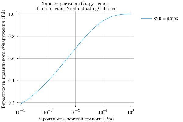
It can be seen from the figure that the point given by Pfa and Pd falls right on the curve. Thus, the SNR corresponding to the ROC curve is the SNR of a single sample at the output of the matched filter. This shows that although multiple samples can be used for detection, the SNR threshold for a single sample (snrthreshold in the programme) does not change compared to the case of a simple sample. There is no change because the threshold value is essentially determined by Pfa. However, the final threshold, T, changes because of the additional gain of the matched filter. The resulting Pfa value remains the same compared to the case where only one sample is used for detection. However, the additional matched gain improved Pd from 0.1390 to 0.3947.

To verify the relationship between Pd, Pfa and SNR, similar calculations can be performed for an incoherent receiver.

Signal detection using pulse integration

Pulse integration is often used in radar and sonar systems to further improve detection performance. If the receiver is coherent, pulse integration is reduced to adding the real parts of the matched filtered pulses. Thus, if a coherent receiver is used, the SNR improvement is linear. If you integrate 10 pulses, the SNR will improve by a factor of 10. For an incoherent receiver, this relationship is not so simple. The following example shows the use of pulse integration with an incoherent receiver.

Assume that the integration is 2 pulses. Then construct the received signal and apply a matched filter to it.

PulseIntNum = 2;
Ntotal = PulseIntNum*Ntrial;
s = wf*exp.(1im*2*pi*rand(rstream,1,Ntotal));  # noncoherent
n = sqrt(npower/2).*(randn(rstream,Nsamp,Ntotal) + 1im*randn(rstream,Nsamp,Ntotal));

If the target is present we get

x = s .+ n;
y = mf'*x;
y = reshape(y,Ntrial,PulseIntNum);  # reshape to align pulses in columns;

Pulse accumulation can be achieved using one of two possible approaches. Both approaches involve approximating a modified Bessel function of the first kind, which is encountered in modelling the likelihood ratio test (LRT) of an incoherent detection process using multiple pulses. The first approach is to sum $|y^2|$ over the pulses, which is often referred to as quadratic law detection. The second approach is to sum $|y|$ over all pulses, which is often referred to as a linear detector. When the ROS is small, a square law detector is preferable, while when the ROS is large, a linear detector is advantageous. In this simulation, we use a square law detector. However, the difference between the two types of detectors is usually within 0.2 dB.

For this example, choose a square law detector, which is more popular than a linear detector. You can use the pulsint function to perform a quadratic law detector. The function treats each column of the input data matrix as a separate pulse. The pulsint function performs the operation

\begin{align} y=\sqrt{|x_1|^2+\cdots+|x_n|^2}\ . \end{align}

z = pulsint(y,"noncoherent");

The relationship between the threshold T and Pfa, given the new sufficient statistic z, is defined as follows

\begin{align} P_{fa}=1-I\left(\frac{T^2/(NM)}{\sqrt{L}},L-1\right) =1-I\left(\frac{\rm SNR}{\sqrt{L}},L-1\right)\ . \end{align}

where \begin{align} I(u,K)=\int_0^{u\sqrt{K+1}}\frac{e^{-\tau}\tau^K}{K!}d\tau \end{align}

is the form of the incomplete Pearson gamma function, and L is the number of pulses used for pulse integration. Using a quadratic law detector, the SNR threshold value associated with pulse integration can be calculated using the npwgnthresh function as before.

snrthreshold = db2pow(npwgnthresh(Pfa,PulseIntNum,"noncoherent"));

The resulting threshold for sufficient statistics, $z$, is defined as follows

mfgain = mf'*mf;
threshold = (sqrt.(npower*mfgain*snrthreshold))[1];

The probability of detection is defined as follows

Pd = sum(z.>threshold)/Ntrial
print("Pd = $(Pd)")

Pd = 0.52807

Then calculate Pfa when the received signal is noise only, using an incoherent detector with integrated 2 pulses.

x = n;
y = mf'*x;
y = reshape(y,Ntrial,PulseIntNum);
z = pulsint(y,"noncoherent");
Pfa = sum(z.>threshold)/Ntrial
print("Pfa = $(Pfa)")

Pfa = 0.00101

To plot the ROC curve with pulse integration, you must specify the number of pulses used in the integration in the rocsnr function:

rocsnr(snrdb_new,SignalType="NonfluctuatingNoncoherent",
    MinPfa=1e-4,NumPulses=PulseIntNum)

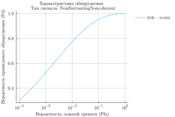
Again, the point given by Pfa and Pd falls on the curve. Thus, the SNR on the ROC curve defines the SNR of one sample used for single pulse detection.

This SNR value can also be obtained from Pd and Pfa using the Albersham equation. The result obtained from the Albersheim equation is only an approximation, but it is good enough over the commonly used Pfa, Pd and pulse integration ranges.

Note: The Albersheim equation has several assumptions:

• the target is non-fluctuating,
• the noise is white Gaussian;
• the receiver is incoherent;
• a linear detector is used for detection.

To calculate the required RMSE for a single sample to achieve a specific Pd and Pfa, use the Albersham function

snr_required = albersheim(Pd,Pfa,N=PulseIntNum)
print("snr_required = $(round(snr_required;digits=5))")

snr_required = 6.01593

This calculated required OSD value corresponds to a new OSD value of 4 dB.

To see the improvement of Pd due to pulse integration, we plot the ROC curve without pulse accumulation.

rocsnr(snrdb_new,SignalType="NonfluctuatingNoncoherent",
    MinPfa=1e-4,NumPulses=1)

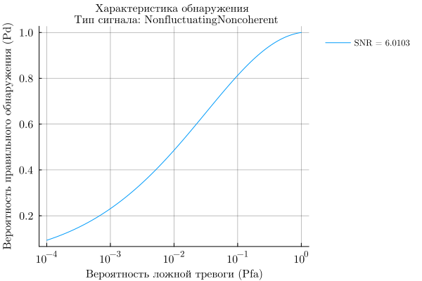
From the figure, it can be seen that without pulse accumulation, the Pd can only be about 0.24 at Pfa 1e-3. When two pulses are accumulated, as shown in the Monte Carlo simulation above, for the same Pfa Pd is about 0.53.

Conclusion

This example has shown how the use of multiple signal sampling in detection can improve the probability of detection while maintaining the desired level of false alarm probability. In particular, it has been shown how the use of a longer signal or pulse accumulation method can improve Pd. An example shows the relationship between Pd, Pfa, the ROC curve and the Albersheim equation. The efficiency is calculated using Monte Carlo simulations.