Beam shaping based on phase shift

This example shows how to apply classical phase shift beamforming to a narrowband signal received by an antenna array. The system model includes the receiver's own noise.

Auxiliary functions

# запуск симуляцик системной модели
function run_model( name_model, path_to_folder ) # определение функции для прогона модели
    Path = path_to_folder * "/" * name_model * ".engee"
    if name_model in [m.name for m in engee.get_all_models()] # Проверка условия загрузки модели в ядро
        model = engee.open( name_model ) # Открыть модель
        model_output = engee.run( model, verbose=true ); # Запустить модель
        engee.close( name_model, force=true ); # Закрыть модель
    else
        model = engee.load( Path, force=true ) # Загрузить модель
        model_output = engee.run( model, verbose=true ); # Запустить модель
        engee.close( name_model, force=true ); # Закрыть модель
    end
    return model_output
end;

# считывание выходных данных
function calc_array_out(out, name)
    array = zeros(eltype(out[name].value[1]),size(out[name].value[1],1),size(out[name].value[2],2),length(out[name].value))
    [array[:,:,i] = collect(out[name].value[i]) for i in eachindex(out[name].value)]
    return array
end

# построение выходных графиков
function plot_result(out, title, number, t_step = 0.3)
    t = Vector(0:t_step/size(out, 1):t_step*(1-1/size(out, 1)))*10^3 # сетка времени в мс
    plot(t, out[:, 1, number], label = title, title = title,size=(500,250))
    plot!(t, out_ref_pulse[:, 1, number], label = "Эталонный сигнал", 
        xlabel = "Время (мс)", уlabel = "Амплитуда (В)"
    )
end;

The figures show the output of a single element (without beamforming) with a reference pulse and the output of the beamformer with a reference pulse. When the received signal is not generated by the beam, the pulse cannot be detected due to noise. The image of the output of the beamformer shows that the signal generated by the beam is much more noisy. The output SNR is about 10 times greater than the signal received by a single antenna, since a 10-element array gives a gain of 10.

1. Description of the model structure

The model simulates the reception of a rectangular pulse with an offset delay on a 10-element uniformly linear antenna array (AR). The pulse source is located in the direction of: azimuth angle of 45 degrees and elevation angle of 0 degrees. 0.5 Watt noise is added to the signal at each element of the grid. Then a beam shaper is applied that takes into account the phase shift between the AR elements. The example compares the output of the beamformer with the signal received by one element of the antenna.

The block diagram of the system is shown below.

The implementation of the system consists of modeling the received signal, receiving the signal, and processing the signal. The following blocks correspond to each stage of the model:

Signal modeling:

Rectangular Pulse Generator (Rectangular) - Creates rectangular pulses.
Delay (Offset waveform) - The delay unit delays each pulse by 150 counts.

Signal reception:

Receiving narrowband radiation using a phased array (Narrowband Rx Array) - simulates the signals received on the AR. The first input to this block is a column vector containing the received pulses. It is assumed that the pulses are narrow-band with a carrier frequency equal to the operating frequency specified in the dialog panel of the unit. The second input "Ang" sets the direction of pulse drop. The antenna array configuration is created in the "Sensor Array" tab of the unit's dialog panel. Each column of the output data corresponds to the signal received on each element of the antenna array.
Receiver Preamp (Receiver Preamp) - implements the pre-amplification of the received AR signal. The unit takes into account the receiver's own thermal noise.
The direction of arrival of the signal (Signal direction) - sets the direction of arrival of the pulses to the block Narrowband Rx Array.

Signal processing:

Direction of beamforming (Angle to beamform) - The Constant block sets the direction of arrival of the signal to the beamformer.
Phase Shift Beamformer (Phase Shift Beamformer) - performs narrow-band beamforming taking into account the phase shift for each element of the antenna array.

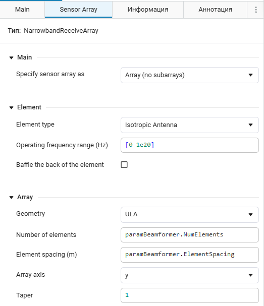
The antenna array characteristics can be set in the Sensor Array tab of the "Phase Shift Beamformer" block. An example of parameterized initialization of a 10-element linear antenna array is shown in the figure below.

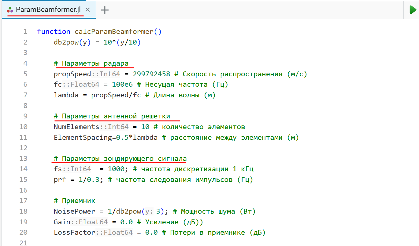
2. Initialization of model parameters

The model parameters are set in the file ParamBeamformar.jl using the auxiliary function calcParamBeamformer. This function is performed once when the model is loaded. It exports a structure to the workspace, the fields of which are referenced by the dialog panels of the model. To change any parameters, either change the values in the structure from the command line, or edit the auxiliary function and restart it to update the parameter structure.

# подключение файла с параметрами модели
include("$(@__DIR__)/ParamBeamformer.jl");

3. Launching the model

Using the function run_model let's run a simulation of the system model Beamformer_with_noise. We will write the generated simulation results into a variable out.

out = run_model("Beamformer_with_noise", @__DIR__) # запуск модели

Building...
Progress 0%
Progress 10%
Progress 100%
Progress 100%

SimulationResult(
    "Эталонный_импульс" => WorkspaceArray{Vector{Float64}}("Beamformer_with_noise/Эталонный_импульс")
,
    "После_формирования" => WorkspaceArray{Matrix{Float64}}("Beamformer_with_noise/После_формирования")
,
    "Без_формирования" => WorkspaceArray{Vector{Float64}}("Beamformer_with_noise/Без_формирования")

)

4. Reading the output data

Using the function calc_array_out counting data from a variable out for each pledged output.

out_ref_pulse = calc_array_out(out, "Эталонный_импульс")
out_beamformer = calc_array_out(out, "После_формирования")
out_not_beamformer = calc_array_out(out, "Без_формирования");

5. Visualization of the results of the model

Visualization of the results is possible in two ways:

in the "graphs" tab (by selecting the "array construction" graph type)
in a script using the data obtained as a result of the simulation

Using the first method, we visualize the result of the model for outputs with and without ray shaping.:

![newplot (1).png](attachment:newplot (1).png)
![newplot (2).png](attachment:newplot (2).png)

The figures show the output of a single element (without beamforming) with a reference pulse and the output of the beamformer with a reference pulse. When the received signal is not generated by the beam, the pulse cannot be detected due to noise.

The situation changes if you use a beamforming algorithm: the lower graph shows that the signal generated by the beam is noticeably more noisy. This result is achieved due to the fact that the output signal-to-noise ratio increases in proportion to the number of antenna elements (approximately 10 times) compared to the signal before the algorithm was used.

Similarly, you can visualize the simulation results using the second method.To build it in the script, use the auxiliary function plot_result:

num_puls = length(collect(out["Эталонный_импульс"]).time) # извлечение номера последнего импульса
plot_result(out_not_beamformer, "Без формирования", num_puls, t_step) |> display
plot_result(out_beamformer, "После формирования", num_puls, t_step)

Comparing the resulting graphs, you can see that the resulting images are identical.

Conclusion

In the example, a beamforming algorithm was considered that takes into account the phase shift between antenna elements ("Phase Shift Beamformer"). Using the algorithm in the receiving path made it possible to successfully project a useful signal against the background of the receiver's own noise.

Blocks used in example¶

Abs