Modeling the microdopler effect

The example introduces the concept of the microdopler effect and demonstrates the construction of a radar system capable of extracting a microdopler from a reflected signal. This feature can be used in the future to solve the problem of goal classification.

Connecting libraries and functions

let
    installed_packages = collect(x.name for (_, x) in Pkg.dependencies() if x.is_direct_dep)
    list_packages = ["DSP","FFTW","LinearAlgebra"]
    for pack in list_packages
        pack in installed_packages || Pkg.add(pack)
    end
end

using DSP,FFTW,LinearAlgebra

gr()
default(titlefontsize=12,top_margin=5Plots.px,guidefont=10,
    fontfamily = "Computer Modern",colorbar_titlefontsize=8,size=(800,400),
    margin = 2Plots.mm
)
function helicopmotion(t,tgtmotion,BladeAng,ArmLength,BladeRate,prf = 2e4, radarpos = [0;0;0])

    Nblades  = size(BladeAng,2)
    tgtpos,tgtvel = tgtmotion(1/prf)

    RotAng = BladeRate*t;
    scatterpos = [0 ArmLength*cos.(RotAng .+ BladeAng);0 ArmLength*sin.(RotAng .+ BladeAng);zeros(1,Nblades+1)].+tgtpos
    scattervel = [0 -BladeRate*ArmLength*sin.(RotAng .+ BladeAng);0 BladeRate*ArmLength*cos.(RotAng .+ BladeAng);zeros(1,Nblades+1)] .+tgtvel

    _,scatterang = rangeangle(scatterpos,radarpos)

    return scatterpos,scattervel,scatterang
end

function spectrogramm_ped(x,t_step;down_lim = -35)

    out,f,t = EngeePhased.Functions.spectrogram(sum(x;dims=1)[:];
        window = DSP.kaiser(128,10),
        noverlap=120,
        nfft=256,fs=1/t_step,
        centered=true,freqloc = "yaxis",out = :data
    )
    out_sig = map(x -> x < down_lim ? down_lim : x,DSP.pow2db.(abs.(out)))
    fig = Plots.heatmap(
        t[:],f,out_sig,color= :jet,
        gridalpha=0.5,
        colorbar_title = "Power, dBW",
        xticks=0:0.5:3,
        yticks=-500:100:500,
    )
    Plots.xlabel!("Time, from")
    Plots.ylabel!("Doppler Frequency, Hz")

    return fig
end

function calc_spectrogram_quad(Data,ts,T;limit = -150)
    x = Data./maximum(abs.(Data))
    dT = T/length(x)
    F = 1/dT

    spec_quad = DSP.spectrogram(x,128,120;window=DSP.kaiser(128,3.95),nfft=512,fs=F)
    power_quad = map(x -> x < limit ? limit : x,pow2db.(spec_quad.power))
    power_quad_quad_new = zeros(size(power_quad))

    power_quad_quad_new[1:round(Int64,size(power_quad,1)/2),:] .= power_quad[round(Int64,size(power_quad,1)/2)+1:end,:]
    power_quad_quad_new[round(Int64,size(power_quad,1)/2)+1:end,:] .= power_quad[1:round(Int64,size(power_quad,1)/2),:]
    fig = Plots.heatmap(spec_quad.time*1e3, fftshift(spec_quad.freq)*1e-3, power_quad_quad_new,color= :jet,
        gridalpha=0.5,ylims=(-10,10),xlims=(0,500),colorbar_title = "Power, dBW",
        xticks=0:50:500,yticks=-10:2:10)
    Plots.xlabel!("Time, ms")
    Plots.ylabel!("Doppler frequency, kHz")
    Plots.title!("Spectrogram of the reflected signal from a helicopter")

    return fig
end


function helperAnnotateSpectrogram(fig)

    Plots.plot!(fig,[20;50],[4;7],linewidth=2,c=:white,lab="",arrow=Plots.Arrow(:close, :tail, 0.5, 1))
    Plots.annotate!(50, 7.5, ("Blade 1", 10, :white, :center),annotationfontfamily="Roboto")
    Plots.plot!(fig,[70;120],[4;5.5],linewidth=2,c=:white,lab="",arrow=Plots.Arrow(:close, :tail, 0.5, 1))
    Plots.annotate!(120, 6, ("Blade 2", 10, :white, :center),annotationfontfamily="Roboto")

    Plots.plot!(fig,[20;50],[-4;-7],linewidth=2,c=:white,lab="",arrow=Plots.Arrow(:close, :tail, 0.5, 1))
    Plots.annotate!(50, -7.5, ("Blade 3", 10, :white, :center),annotationfontfamily="Roboto")
    Plots.plot!(fig,[70;120],[-4;-5.5],linewidth=2,c=:white,lab="",arrow=Plots.Arrow(:close, :tail, 0.5, 1))
    Plots.annotate!(120, -6, ("Blade 4", 10, :white, :center),annotationfontfamily="Roboto")

    Plots.plot!(fig,[0;250],[0;-0.1],linewidth=3,c=:white,lab="",arrow=Plots.Arrow(:close, :both, 0.5, 1))
    Plots.annotate!(120, -1, ("Period", 10, :white, :center),annotationfontfamily="Roboto")

    Plots.plot!(fig,[124;125],[0.2;4],linewidth=3,c=:white,lab="",arrow=Plots.Arrow(:close, :both, 0.5, 1))
    Plots.annotate!(137, 2, ("Rotation speed", 10, :white, :left),annotationfontfamily="Roboto")

end


function plotting_svd(x)
    Plots.plot(10*log10.(x),lab="",ylabel="Singular values",xlabel="rank")
    Plots.plot!([55], seriestype="vline", label="",ls=:dashdot,color="red",lw=2)
    Plots.plot!([101], seriestype="vline", label="",ls=:dashdot,color="red",lw=2)
    Plots.plot!([109], seriestype="vline", label="",ls=:dashdot,color="red",lw=2)
    Plots.annotate!(25, -10, ("A", 10, :black, :left),annotationfontfamily="Roboto")
    Plots.annotate!(75, -10, ("B", 10, :black, :left),annotationfontfamily="Roboto")
    Plots.annotate!(102, -10, ("C", 10, :black, :left),annotationfontfamily="Roboto")
    Plots.annotate!(175, -10, ("D", 10, :black, :left),annotationfontfamily="Roboto")
end

plotting_svd (generic function with 1 method)

1. The concept of the microdopler effect

The concept of micro-movements is inextricably linked with the microdopler effect*:

Micro–movement is a slight movement or deviation of a component part of an object, which is additional to the main volumetric movement of the whole object [1]. The source of micro-motion can be a vibrating surface, rotating rotor blades of a helicopter, a walking person making periodic movements with his arms and legs, flapping wings of a bird, or other reasons.

The microdopler effect is a phenomenon associated with the enrichment of the spectral composition of the reflected signal, which occurs during radar research as a result of micro-movements of objects.

Let's consider 2 scenarios for the movement of an object: a simple translational movement (top picture) and a complex translational-rotational movement (bottom picture).

In case 1, the object is moving towards us uniformly, so the Doppler frequency has a constant value, independent of time.

In the second case, the situation changes: rotational motion (for example, the rotation of helicopter blades) introduces periodically changing components into the spectrum of the reflected signal, which characterize the microdopler effect.

A spectrogram of a reflected signal containing Microdopler components in the spectrum is called Microdopler signatures (or abbreviated as MDS). An example of a bird's MDS is given below:

2. Simulation of pedestrian MDS

In the next section, we will consider the creation of an automotive radar based on a continuous signal from an LFM to identify a crossing on the road.

2.1 Descriptions of the model scenario

The model considers the following scenario:

a car with a radar is moving along the inside lane at a speed of 30 km/h from the origin towards a parked car and a pedestrian;
The parked car is located at a distance of 39.4 m
The pedestrian is moving at a speed of 1 m/s

A visualization of the scenario is given below:
Пешеход с двумя автомобилями (2).png

2.2 Model Parameters

High range and speed resolution is required to identify the transition. In automotive radars, a continuous linear frequency modulated (FM) signal is used to meet the characteristics.

bw = 250e6 # signal band, Hz
fs = bw # sampling rate, Hz
fc = 24e9 # carrier frequency, Hz
tm = 1e-6 # scan time, s
c = 3e8 # speed of light, m/s

egocar_pos = [0;0;0] # m, the position vector of the car with radar
egocar_vel = [30*1600/3600;0;0] # m/s, the speed vector of a car with radar

parkedcar_pos = [39;-4;0] # m, the vector of the position of the car in front
parkedcar_vel = [0;0;0] # m/s, the velocity vector of the car in front

ped_pos = [40;-3;0] # m, the vector of the pedestrian's position
ped_vel = [0;1;0] # m, pedestrian velocity vector
ped_heading = 90 # hail, the pedestrian's initial direction of movement
ped_height = 1.8; # pedestrian height

2.3 Formation of system objects

To formalize the reflected signal of a pedestrian object, use the system objects EngeeRadars.BackscatterPedestrian

wav_fmcw = EngeePhased.FMCWWaveform(
    SampleRate=fs, # sampling rate
    SweepTime=tm, # scan time
    SweepBandwidth=bw # signal band
)

# From a car with radar
egocar = EngeePhased.Platform(
    InitialPosition=egocar_pos, # starting position
    Velocity=egocar_vel, # velocity vector
    OrientationAxesOutputPort=true # enabling the spatial orientation output port
)

# The formation of the object in front of the car
parkedcar = EngeePhased.Platform(
    InitialPosition=parkedcar_pos, # starting position
    Velocity=parkedcar_vel, # speed
    OrientationAxesOutputPort=true # enabling the spatial orientation output port
)
parkedcar_tgt = EngeePhased.RadarTarget(PropagationSpeed=c,OperatingFrequency=fc,MeanRCS=10)

# Pedestrian object formation
ped = EngeeRadars.BackscatterPedestrian(
    InitPosition=ped_pos, # starting position
    InitHeading=ped_heading, # the initial direction of movement
    PropagationSpeed=c, # signal propagation speed
    OperatingFrequency=fc, # carrier frequency
    Height=ped_height, # height
    WalkingSpeed=1 # The speed of movement
)

# Distribution channels: to the pedestrian and the nearest car
chan_ped = EngeePhased.FreeSpace(
    PropagationSpeed=c, # The speed of propagation
    OperatingFrequency=fc, # carrier frequency
    TwoWayPropagation=true, # accounting for bidirectional propagation
    SampleRate=fs # sampling rate
)
chan_pcar = EngeePhased.FreeSpace(
    PropagationSpeed=c, # The speed of propagation
    OperatingFrequency=fc, # carrier frequency
    TwoWayPropagation=true, # accounting for bidirectional propagation
    SampleRate=fs # sampling rate
)

# receiver and transmitter
tx = EngeePhased.Transmitter(PeakPower=1,Gain=25)
rx = EngeePhased.ReceiverPreamp(Gain=25,NoiseFigure=10);

2.4 Simulation of the model

For the correct display of the pedestrian's MDS, it is necessary to accumulate the reflected signal during at least one cycle of human movement. The pedestrian's speed is 1 m/s, so it takes 2 seconds to complete the cycle. Let's simulate a pedestrian movement scenario for 2.5 seconds in 1 ms increments.:

Tsim = 2.5 # Simulation time
Tsamp = 0.001 # simulation calculation step, with
npulse = round(Int64,Tsim/Tsamp) # number of pulses
# Memory allocation under:
xr = complex(zeros(round(Int64,fs*tm),npulse)) # total reflected signal
xr_ped = complex(zeros(round(Int64,fs*tm),npulse)) # reflected signal from pedestrian
@inbounds for m = 1:npulse
    # calculation of current position, speed, orientation and viewing angle
    # to a pedestrian and a parked car
    pos_ego,vel_ego,ax_ego = egocar(Tsamp)
    pos_pcar,vel_pcar,ax_pcar = parkedcar(Tsamp)
    pos_ped,vel_ped,ax_ped = move(ped,Tsamp,ped_heading)
    _,angrt_ped = rangeangle(pos_ego,pos_ped,ax_ped)
    _,angrt_pcar = rangeangle(pos_ego,pos_pcar,ax_pcar)

    # calculation of the reflected signal
    global x = tx(wav_fmcw()) # probing signal
    # transmission of signals in the forward and reverse propagation channel
    xt_ped = chan_ped(repeat(x,1,size(pos_ped,2)),pos_ego,pos_ped,vel_ego,vel_ped)  
    xt_pcar = chan_pcar(x,pos_ego,pos_pcar,vel_ego,vel_pcar)
    xt_ped = reflect(ped,xt_ped,angrt_ped) # reflected signal from the transition
    xt_pcar = parkedcar_tgt(xt_pcar) # reflected signal from the car
    xr_ped[:,m] = rx(xt_ped) # received signal from pedestrian
    xr[:,m] = rx(xt_ped+xt_pcar) # received signal from pedestrian
end

# transferring the signal to the zero frequency
xd_ped = conj(dechirp(xr_ped,x))
xd = conj(dechirp(xr,x));

2.5 Processing of the received signal

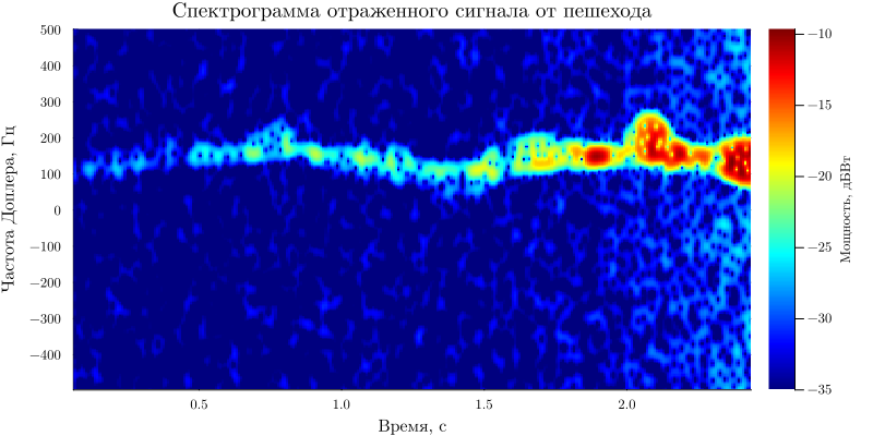
In the simulated signal xd_ped it contains only the pedestrian's response, and xd It contains the response of both a pedestrian and a parked car. If we create a spectrogram using only the reflected signal from a pedestrian, we get the following MDS:

spectrogramm_ped(xd_ped,Tsamp;down_lim = -35)
title!("A spectrogram of the reflected signal from a pedestrian")

The spectrogram of the total reflected signal from a pedestrian and a car looks like this:

spectrogramm_ped(xd,Tsamp;down_lim = -35)
title!("Spectrogram of reflected signal from pedestrian and car")

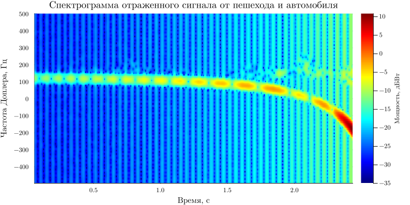
It can be noted that the vehicle's MDS dominates the pedestrian's MDS. Therefore, a pedestrian cannot be detected without additional processing.

2.6 SVD decomposition processing

To detect a weaker signal based on a strong one, you can use singular value decomposition to identify the area of interest.

out_svd = svd(xd,full=true) # calculation of the decomposition component
uxd,sxd,vxd = out_svd.U,out_svd.S,out_svd.V; # reading the S,U,V matrices

Using the function plotting_svd let's display the main diagonal singular matrix S:

plotting_svd(sxd)

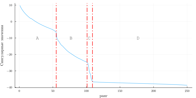
On the graph of the dependence of the signal values on the rank of the matrix, 4 areas can be conditionally distinguished:

A - includes the main signal, which makes a significant contribution to the spectrogram;
B - a combination of pedestrian and car signals, with the dominance of the second
C - a combination of pedestrian and car signals, with the former dominating;
D is the noise contribution of the receiving device.

Therefore, in order to effectively isolate the pedestrian's MDS, it is necessary to extract from the entire spectrogram the area C located within the range of the rank 103-110:

rk = 103:110 # the range of ranks of the matrix of signular values

# calculation of the processed spectrogram
sxd_new = [sxd;zeros(size(vxd,1)-length(sxd))]
xdr = uxd[:,rk]*Diagonal(sxd_new)[rk,:]*vxd';

We will build the pedestrian and car MDS again after additional processing (for correct display, we will reduce the lower limit to -40 dB since the main power has been removed):

spectrogramm_ped(xdr,Tsamp;down_lim = -40)
title!("MDS of pedestrian and car after SVD transformation")

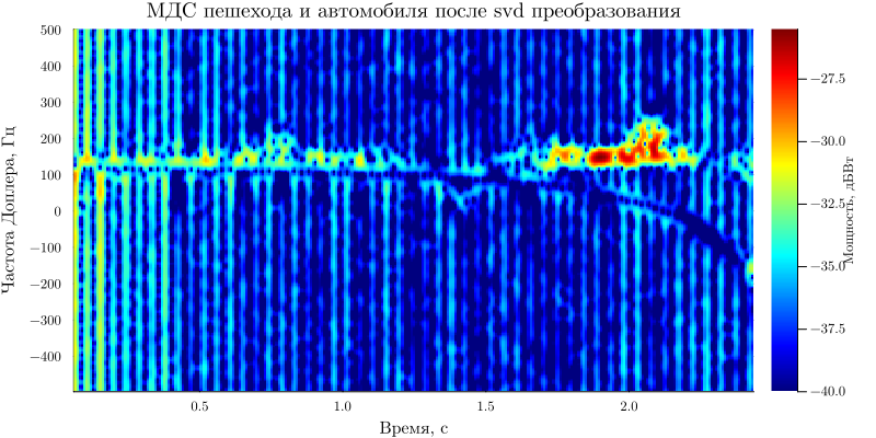
After filtering the signal from the car, a clear picture of the pedestrian's MDS is formed, while the level of the car's MDS has significantly decreased.

Thus, with the help of additional processing (svd decomposition), it was possible to isolate the spectral components of a pedestrian against the background of an interfering signal from a nearby car.

3. Helicopter MDS simulation

3.1 Description of the model scenario

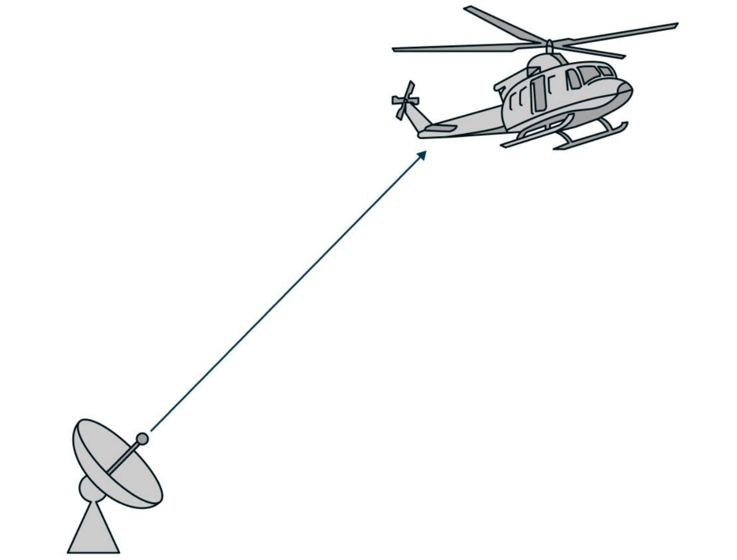
Consider the case:

The helicopter flies at a distance of [-25,500,500] meters evenly in the x-z plane at a speed of 100 m/s along the x axis.
The radar is stationary and located at the origin.
In this case, at the beginning of the movement, the helicopter approaches the radar, and after moving to the positive area of the x-axis, it will begin to move away. A visualization of this scenario is given below:

3.2 Model parameters

Let's set the parameters of the radar and target (helicopter) movement scenario:

radarpos = [0;0;0] # radar position vector, m
radarvel = [0;0;0] # radar velocity vector, m/s

tgtinitpos = [-25;500;500] # the initial position of the target, m
tgtvel = [100;0;0]; # target speed, m/s

Next, we will form the geometry of the helicopter, specifying its main parameters (number of blades, length of blades, speed of rotation of the propeller):

f_rot = 4 # screw rotation speed, c
Nblades   = 4 # number of blades
bladeang  = Matrix((0:Nblades-1)')*2*pi/Nblades # вектор углов лопастей
bladelen  = 6.5 # blade length, m
bladerate = deg2rad(360*f_rot);  # The rotation speed of the screw is rad/s

25.132741228718345

The next stage is the formation of a radar station. Let's set the fundamental parameters of the system:

c  = 3e8 # signal propagation speed, m/s
fc = 5e9 # carrier frequency, Hz
fs = 1e6 # sampling rate, Hz
prf = 2e4 # pulse repetition rate, Hz
lambda = c/fc; # wavelength, m

3.3 Creating system objects

Now, using the parameters of the target scenario and the radar system, we will create system model objects using the library EngeePhased:

# Goal formation
helicop = EngeePhased.RadarTarget(
    MeanRCS=[10 .1 .1 .1 .1], # EPR of helicopter elements (fuselage and 4 blades)
    PropagationSpeed=c, # The speed of propagation
    OperatingFrequency=fc # carrier frequency of the signal
)
tgtmotion  = EngeePhased.Platform(InitialPosition=tgtinitpos,Velocity=tgtvel)

# Probing signal generator
wav = EngeePhased.RectangularWaveform(
    SampleRate=fs, # sampling rate
    PulseWidth=2/fs, # pulse duration
    PRF=prf # pulse repetition rate
)
# Antenna array formation (rectangular 4x4)
ura = EngeePhased.URA(
    Size=[4 4], # antenna array size
    ElementSpacing=[lambda/2 lambda/2] # the distance between the elements
)
tx  = EngeePhased.Transmitter() # The transmitter
rx  = EngeePhased.ReceiverPreamp() # The preamp

# Distribution environment
env = EngeePhased.FreeSpace(
    PropagationSpeed=c, # propagation velocity, m/s
    OperatingFrequency=fc, # carrier frequency, Hz
    TwoWayPropagation=true, # accounting for bidirectional propagation
    SampleRate=fs # sampling rate
)
# Transmitting AR
txant = EngeePhased.Radiator(
    Sensor=ura, # AR geometry
    PropagationSpeed=c, # propagation velocity, m/s
    OperatingFrequency=fc # carrier frequency, Hz
)
# The receiving AR
rxant = EngeePhased.Collector(
    Sensor=ura, # AR geometry
    PropagationSpeed=c, # propagation velocity, m/s
    OperatingFrequency=fc # carrier frequency, Hz
);

3.4 Running a simulation of the model

We implement the calculation of the radar operation scenario when the helicopter is moving by calling system objects in a loop.:

NSampPerPulse = round(Int64,fs/prf) # the number of samples in 1 pulse
Niter = Int64(1e4) # number of iterations (number of pulses emitted)
y = complex(zeros(NSampPerPulse,Niter)) # memory allocation for the reflected signal

@inbounds for m in 1:Niter
    # Helicopter position and speed update
    t = (m-1)/(prf) # time simulation step
    global scatterpos,scattervel,scatterang = helicopmotion(t,tgtmotion,bladeang,bladelen,bladerate,prf,radarpos)

    # calculation of the reflected signal
    x  = txant(tx(wav()),scatterang)  # probing signal
    xt = env(x,radarpos,scatterpos,radarvel,scattervel) # Wednesday's signal
    xt = helicop(xt) # reflected signal from helicopter
    global xr = rx(rxant(xt,scatterang)) # received signal
    y[:,m] = sum(xr;dims=2) # beam formation
end

3.5 Signal processing

Using a system object RangeDopplerResponse we implement range-Doppler processing:consistent range filtering and spectral processing based on speed FFT.

rdresp  = EngeePhased.RangeDopplerResponse(
    PropagationSpeed=c, # signal propagation speed
    SampleRate=fs, # sampling rate
    DopplerFFTLengthSource="Property", # The method of setting the FFT (in the CO parameters)
    DopplerFFTLength=128, # FFT length
    DopplerOutput="Speed", # Doppler output (speed)
    OperatingFrequency=fc # carrier frequency
)

mfcoeff = getMatchedFilter(wav)
fig1 = plotResponse(rdresp,y[:,1:128],mfcoeff)
Plots.ylims!(0,3000)
Plots.plot!(fig1,title="Range-Doppler portrait",xlabel="Speed, m/s",
    ylabel="Range, m",titlefontsize=12,top_margin=5Plots.px,guidefont=10,
    colorbar_title="Power, dBW",fontfamily = "Computer Modern",colorbar_titlefontsize=8)

It can be noted that the range-Doppler portrait captures the presence of 3 components: the central component is the fuselage of the helicopter, and the lateral components are the rotation of the blades.

Let's estimate the radial velocity of the helicopter:

tgtpos = scatterpos[:,1] # the helicopter's position at the end of the simulation
tgtvel = scattervel[:,1] # helicopter speed at the end of the simulation
tgtvel_truth = radialspeed(tgtpos,tgtvel,radarpos,radarvel)
println("radial velocity of the helicopter fuselage $(round(tgtvel_truth;sigdigits=3)) m/s")

радиальная скорость фюзеляжа вертолета -3.53 м/с

We will also look at the maximum and minimum values of the radial speeds of the screws.:

maxbladetipvel = [bladelen*bladerate;0;0] # the speed of the propeller blades
vtp = radialspeed(tgtpos,-maxbladetipvel+tgtvel,radarpos,radarvel)
vtn = radialspeed(tgtpos,maxbladetipvel+tgtvel,radarpos,radarvel)
println("maximum radial velocity value $(round(vtp;sigdigits=3)) m/s")
println("minimum radial velocity value $(round(vtn;sigdigits=3)) m/s")

максимальное значение радиальной скорости 2.24 м/с
минимальное значение радиальной скорости -9.3 м/с

Let's perform consistent filtering and construct a spectrogram of the reflected signal.:

# Consistent filtering
mf  = EngeePhased.MatchedFilter(Coefficients=mfcoeff) # consistent filter
ymf = mf(y) # processing
ridx = findmax(sum(abs.(ymf);dims=2)[:])[2]; # range peak detection

# Building an MDS
T = Niter/prf # duration of the spectrogram
fig1 = calc_spectrogram_quad(ymf[ridx,:],1/prf,T;limit=-100)

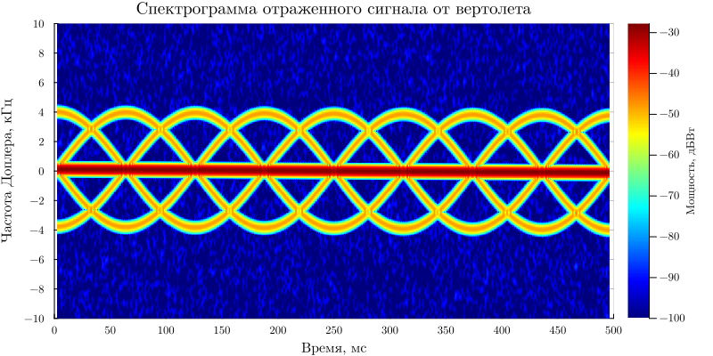
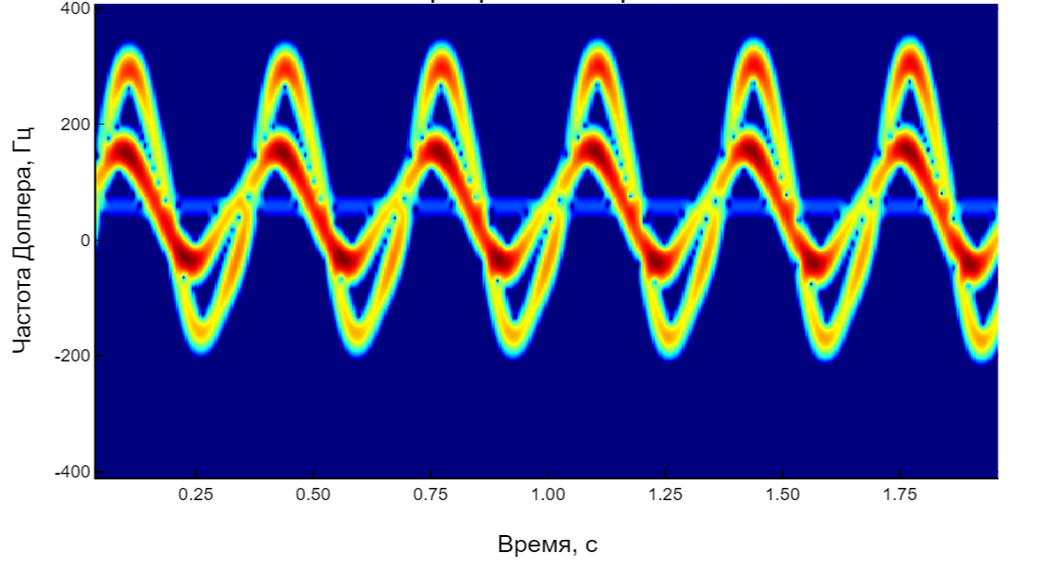
The central component characterizes the reflected signal from the helicopter fuselage, the periodic components are the rotation of the blades. We visualize the components of the MDS using the function helperAnnotateSpectrogram:

helperAnnotateSpectrogram(fig1)

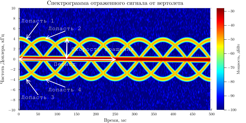
The oscillation period, which is approximately 250 ms, can be estimated from the graph of the spectrogram. In this case, the estimated number of blades is:

Tp = 250e-3 # the MDS period
bladerate_est = 1/Tp # estimating the number of blades
println("Estimation of the number of blades $(round(bladerate_est;sigdigits=2))")

Оценка числа лопастей 4.0

The maximum deviation of the Doppler frequency is approximately 4 kHz, then the radial velocity of the helicopter blades is estimated as:

f_doppler = 4e3 # the amplitude of the Doppler frequency, Hz
Vt_detect = dop2speed(f_doppler,lambda)/2
println("Radial velocity of the blades $(Vt_detect) m/s")

Радиальная скорость вертолета 120.0 м/с

To estimate the true speed, it is necessary to determine and solve the pelingation problem based on the angle of the location. Let's use the "Music" algorithm implemented in the system object. MUSICEstimator2D:

doa = EngeePhased.MUSICEstimator2D(
    SensorArray=ura, # 
    OperatingFrequency=fc, # carrier frequency
    PropagationSpeed=c, # signal propagation speed
    DOAOutputPort=true, # turning on the angular direction output
    ElevationScanAngles=-90:90 # scanning range by location angle
)
_,ang_est = doa(xr) # calculation of viewing angles
Vt_est = Vt_detect/cosd(ang_est[2]) # estimating the speed of the blades
println("Blade velocity estimate $(round(Vt_est;sigdigits=3)) m/s")

Оценка скорости лопастей 170.0 м/с

Knowing the estimates of the speed and number of blades, we will determine the approximate length of the blade.:

bladelen_est = Vt_est/(bladerate_est*2*pi)
println("Blade length estimate $(round(bladelen_est;sigdigits=3)) m")

Оценка длины лопасти 6.75 м

The true length value is 6.5 m, hence the error was 4%.

Conclusion

In the example, the concept of the "microdopler effect" and Microdopler signatures is considered. Using the EngeePhased system objects, MDS reflected signals were modeled for 2 radar scenarios: a ground-based radar in the presence of an aerial target - a helicopter and an automobile radar in the presence of a pedestrian and a nearby car.