Modeling and visualization of range and Doppler frequency data in a radar system with multiple targets
This example demonstrates how to model a radar system and use the calc_range_dopper_visual function to visualize range and Doppler intensity data over time in Engee. Range-time and Doppler-time intensity meters help detect a target in the environment by showing how the target's range and Doppler parameter change over time.
Functions used
# function for running the model
function run_model( name_model, path_to_folder )
    Path = path_to_folder * "/" * name_model * ".engee"
    if name_model in [m.name for m in engee.get_all_models()] # Checking the condition for loading a model into the kernel
        model = engee.open( name_model ) # Open the model
        model_output = engee.run( model, verbose=true ); # Launch the model
        # engee.close( name_model, force=true ); # Close the model
    else
        model = engee.load( Path, force=true ) # Upload a model
        model_output = engee.run( model, verbose=true ); # Launch the model
        # engee.close( name_model, force=true ); # Close the model
    end
    return model_output
end;

# the function of constructing dynamic visualization of changes in Doppler range and frequency
function calc_range_doppler_visual(out_range,out_doppler,time_simulation,paramRadarVisual)
    gr()
    out_doppler .= 20log10.(out_doppler .+ eps(1.0))
    max_doppler = maximum(out_doppler)
    out_doppler.= map(x-> x> max_doppler-5 ? x : max_doppler-5,out_doppler)
    num_step = ceil(Int64,size(out_range,3)/20) # The counting step in the simulation

    # Allocating memory to fill simulation data
    viz_Range = fill(NaN,size(out_range)...)
    viz_Doppler = fill(NaN,size(out_doppler)...)

    # Setting axes for building a dynamic graph
    x_axis_range = Vector(range(start=0,stop=paramRadarVisual.max_range,length=size(viz_Range,1)))
    y_axis_range = Vector(range(start=0,stop=time_simulation,length=size(viz_Range,3)))
    x_axis_doppler = Vector(range(start=paramRadarVisual.DopplerOff,
        stop=-paramRadarVisual.DopplerOff,length=size(viz_Doppler,1)))
    y_axis_doppler = Vector(range(start=0,stop=time_simulation,length=size(viz_Doppler,3)))

    plot_range = heatmap(ylabel="Time,from", xlabel="Range, m",font_family="Computer Modern",
        title="Changing the target range over time",title_font=font(12,"Computer Modern"),
        colorbar_title="Power, MCW",color=:viridis,size = (600,400))
    plot_doppler = heatmap(ylabel="Time,from", xlabel="Doppler Frequency, Hz",font_family="Computer Modern",
        title="Changing the Doppler frequency of targets over time",title_font=font(12,"Computer Modern"),
        colorbar_title="Power, dBW",color=:viridis,size = (600,400))

    @info "Building a visualization of changes in target range from time to time..."

    anim1 = @animate for i in 1:num_step:size(viz_Range,3)
        @info "$(round(100*i/size(viz_Range,3))) %"
        viz_Range[:,:,1:i] .= out_range[:,:,1:i]*1e6
        heatmap!(plot_range,x_axis_range,y_axis_range,permutedims(viz_Range[:,1,:]),colorscale= :haline)
        (i+num_step > size(viz_Range,3)) && (heatmap!(plot_range,x_axis_range,y_axis_range,
            permutedims(out_range[:,1,:]*1e6),colorscale= :haline); @info "100.0 %")
    end
    @info "Building a visualization of the Doppler frequency variation over time ..."
    anim2 = @animate for i in 1:num_step:size(viz_Doppler,3)
         @info "$(round(100*i/size(viz_Doppler,3))) %"
        viz_Doppler[:,:,1:i] .= out_doppler[:,:,1:i]
        heatmap!(plot_doppler,x_axis_doppler,y_axis_doppler,permutedims(viz_Doppler[:,1,:]),colorscale= :haline)
        (i+num_step > size(viz_Doppler,3)) && (heatmap!(plot_doppler,x_axis_doppler,y_axis_doppler,
            permutedims(out_doppler[:,1,:]),colorscale= :haline); @info "100.0 %")
    end
    return anim1,anim2
end;
1. Description of the model structure
Let's take a closer look at the structural scheme of the model:
The transmitter (Transmitter)
- Waveform Rectangular: A probe signal source that generates a sequence of rectangular pulses;
- Transmitter: an amplifier of the generated rectangular pulse;
- Narrowband TX Array: transmitting antenna element (or antenna array) forming a directional pattern;
Movement of objects (Platform)
The subsystem of the platform simulates the movement of the radar, as well as targets. The positions and speeds of the radar and targets are used by the Free Space block to simulate propagation and by the Range Angle block to calculate the angles of incidence of the signal at the target location.
- Radar Platform: Used to simulate radar movement. The radar is mounted on a stationary platform located at the origin.
- Target Platform: Used to simulate target movement.
- Range Angle: Used to simulate target movement.
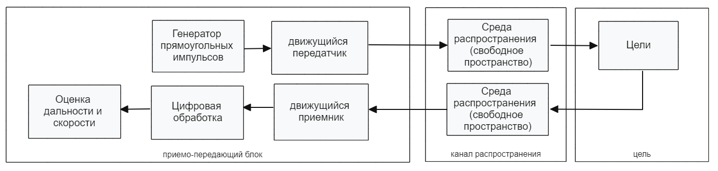
Channel and Targets </h4>
- Free Space: the free space in which the signal propagates to the targets and back to the receiver, undergoing attenuation proportional to the distance to the targets;
- Target: A target model that reflects the incident signal according to the radar cross-section (RCS).
- Receiver (Receiver Preamp): The signal reflected from the targets arrives at the receiving antenna array and is amplified by adding the receiver's own thermal noise.
Receiver (Receiver)
- Narrowband Rx Array: Simulates the signals received by the antenna.
- Receiver Preamp - amplifies the received signal from the target and adds its own thermal noise.
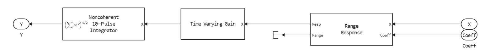
- Range Processing Subsystem - Performs consistent filtering to improve SNR, then the block (Time Varying Gain) performs tunable gain to compensate for range loss and integrates 10 pulses incoherently.
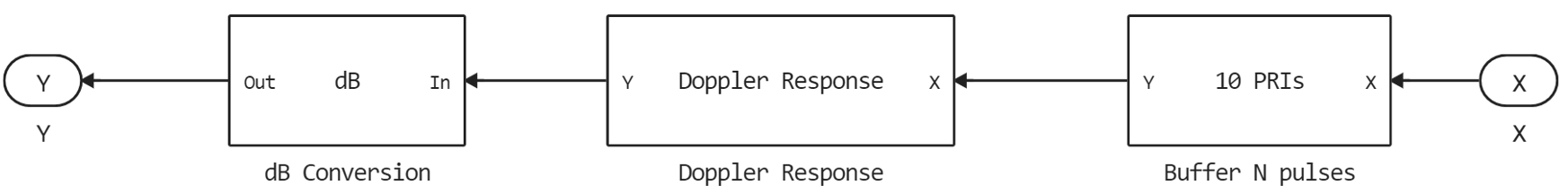
Doppler Processing Subsystem - The received signal accumulates 10 pulses per packet, followed by an FFT to estimate the Doppler frequency (speed) of targets.
The model's operation scheme is shown in the figure below.:
.png)
Digital processing consists of the following elements:
Based on the block diagram, we have developed the radar model shown in the figure below.
.png)
2. Initialization of input parameters
To initialize the input parameters of the model, we will connect the file "ParamRadarVisual.jl". If you need to change the parameter values, then open this file and edit the necessary parameters.
include("$(@__DIR__)/ParamRadarVisual.jl")
paramRadarVisual = calcParamRadarVisual();
pulse_length = paramRadarVisual.pulse_length*100; # Pulse duration
Flexible configuration of the antenna array of the transmitter and receiver is possible in the model, including: element type, antenna array geometry (the model uses 1 isotropic radiator, as shown below):
.png)
3. Launching the model
Define the run function of the model run_model and run the simulation of the model:
run_model("RadarSystemVisualExample", @__DIR__);
The simulation results can be visualized using the graph type ** "Intensity diagram"**:
.png)
On the graph of the range-time diagram, you can see 3 targets: one is approaching the radar, the second is moving away, and 3 are standing still. Also, an estimate of the Doppler frequency is observed on the range-Doppler diagram.
The result of dynamic visualization is shown in the video "VizualizeDiagramm.gif"
4. Reading the output data
We count the necessary variables from the workspace (in our case Range and Doppler):
out_Range = zeros(Float64,size(Range.value[1],1),size(Range.value[2],2),length(Range.value))
[out_Range[:,:,i] = collect(Range.value[i]) for i in eachindex(Range.value)]

out_Doppler = zeros(Float64,size(Doppler.value[1],1),size(Doppler.value[2],2),length(Doppler.value))
[out_Doppler[:,:,i] = collect(Doppler.value[i]) for i in eachindex(Doppler.value)]

time_simulation = Range.time[end];
5. Displaying the results
Using the previously calculated data, we will build a visualization of the system's response by Doppler range and frequency. To do this, call the calc_range_dopper_visual function.:
# saving animations in anim_range,anim_doppler variables
anim_range,anim_doppler = calc_range_doppler_visual(out_Range,out_Doppler,time_simulation,paramRadarVisual)
# Saving the visualization of the response in a format file.gif
gif(anim_range, "Visual_Range.gif", fps = 1)
gif(anim_doppler, "Visual_Doppler.gif", fps = 1);
After saving the files, 2 Visual_Range files will appear in the contents of the current folder.gif and Visual_Doppler.gif , which store the dynamics of Doppler range and frequency changes over time:
.png)
Examples of visualization are given below:
gif(anim_range, "Visual_Range.gif", fps = 1)
gif(anim_doppler, "Visual_Doppler.gif", fps = 1)
Conclusion
As a result, this example demonstrated the design of a radar system in the Engee environment, as well as the calculation and visualization of information about the range and Doppler frequency changing over time.