Modeling of automatic control systems using object models
The model of the automatic control system (ACS) is presented in the form of a block diagram. It contains blocks that describe the dynamics of individual objects. For example, the actuator, sensors, and controllers. In this article, we will consider the functions for working with the ACS model. We will define ways to set object models, some functions for structural transformations and the construction of time characteristics.
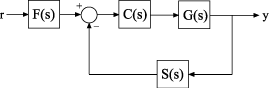
Let's consider the structural scheme of the ACS, which contains filter blocks , a management object , controller and the sensor .
Engee uses the ControlSystems.jl library to work with control systems.
Pkg.add(["ControlSystems"])
# Connecting the library
using ControlSystems
Each of the system components can be represented as an object model. For example, a management object set as a gain factor with a double pole in s=-1 using the function zpk(). The controller indicated by , represented as a PID controller using the function pid(). Models and can be specified as transfer functions using tf().
G = zpk([], [-1, -1], 1)
C = pid(2, 1.3, 0.3; Tf = 0.5)
S = tf(5, [1, 4])
F = tf(1, [1, 1])
The specified transfer functions of the circuit elements can be combined with each other. For example, we obtain the transfer function of an open system using the operator *.
op = C*G*S
To construct the transfer function of a closed system, we use the function feedback().
cl = feedback(C*G,S)
We obtain the transfer function of the entire system, taking into account the filter . To do this, use the function series().
W = series(cl, F)
All the received functions can be analyzed using the ControlSystems.jl library. For example, let's look at the time characteristics. We construct the transition characteristic of the system using the function step(), and the impulse response using impulse().
# Connecting the library for charting
using Plots

ht = step(W,30)
plot(ht, title="Transitional function", label="h(t)")
# Building an impulse response
kt = impulse(W,30)
plot(kt, title="Pulse function", label="k(t)")
There are other functions for analyzing models of automatic control systems in the ConrtrolSystems.jl library. They can be studied in the section [Analysis of time and frequency characteristics] (https://engee.com/helpcenter/stable/julia/ControlSystems/lib/timefreqresponse.html ).