Approximation of the time delay in an open-loop continuous model
This example shows how to approximate delays in an open continuous time system using pade.
The Pad approximation is useful when using analysis or design tools that do not support time delays. Using too high an approximation order can lead to numerical errors and possibly unstable poles. Therefore, avoid approximations of the same order. .
Setting the task
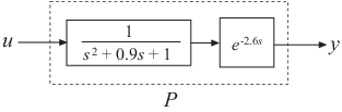
Create a sample of an open-loop system with delayed output.
Pkg.add(["ControlSystems"])
using ControlSystems
By default, the delay is 2.6, but you can set your own parameter. As a result, you will get a P-object in the form of a state space (ss) with a time delay of 2.6 seconds.
s = tf('s');

L = 2.6 # @param {type:"slider", min:0, max:9, step:0.1}
P = exp(-L*s)/(s^2+0.9*s+1)
First-order approximation
Calculate the first-order Pade approximation for P.
Pnd1 = pade(P,1)
This command replaces all time delays in P with a first-order approximation. Thus, Pnd1 is a third—order system without delays.
Compare the frequency response of the initial and approximate models using bodeplot.
bodeplot([P, Pnd1], label = ["P" "Pnd1"])
The amplitude characteristics of P and Pnd1 are exactly the same. However, the Pnd1 phase differs from the P phase by about 1 rad/s.
Third-order approximation
Increase the Pad approximation order to expand the frequency range for which the phase approximation is good.
Pnd3 = pade(P,3);
Compare the frequency characteristics of P, Pnd1 and Pnd3.
bodeplot([P, Pnd1, Pnd3], label = ["P" "Pnd1" "Pnd3"])
The error of the phase characteristic decreases when using the Padet approximation of the third order.
Compare the transient characteristics of the original and approximated systems in the time domain using step.
plot(
    [step(P), step(Pnd1), step(Pnd3)],
    label = ["P" "Pnd1" "Pnd3"]
)
Conclusions
The use of the Pade approximation leads to the appearance of a non-minimal phase in the initial transition process. This effect is quite pronounced in the first-order approximation, which drops significantly below zero before changing direction. In a higher-order approximation, this effect is reduced, and it better matches the exact response of the system.