Smith's Predictor
In this example, an object management system with a long time delay is being developed. To control objects with a delay, the Smith predictor is often used, which can predict which signal should appear at the output of an object before it actually appears there [1].
Pkg.add(["ControlSystems", "ControlSystemsBase"])
using ControlSystemsBase, Plots
using ControlSystems # A library for modeling a delay system
The control object is defined by the equation: , where .
P0 = ss(-1, 1, 1, 0) # Control object without delay
By changing the delay value t, you can see how the system will behave with different delays.
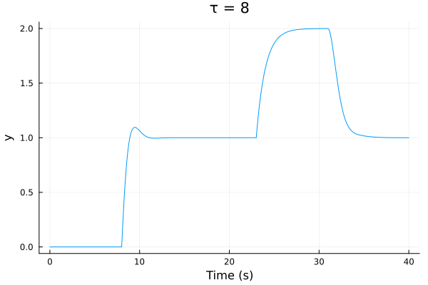
τ = 8 # The amount of delay
P = delay(τ) * P0 # Delayed control object
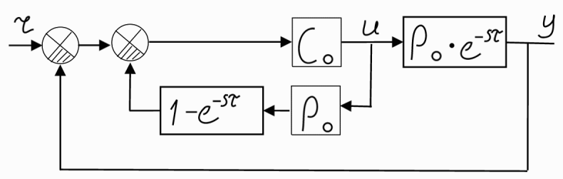
The block diagram of the Smith predictor control system is shown in the figure below. It contains an additional internal feedback loop, which contains the model of the control object. An additional circuit generates a signal identical to the one that eventually appears at the output of the system and feeds it to the input of the regulator until there is a signal from the main feedback circuit. [2]
As a regulator we use a PI controller.
ω0 = 2
ζ  = 0.7
C0, _ = placePI(P0, ω0, ζ) # The PI controller
Smith's Predictor :
C = feedback(C0, (1.0 - delay(τ))*P0) # Formation of internal feedback
Let's build a transition process.
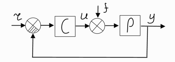
Transfer function for disturbing effect f:
= feedback(P, C).
Transfer function of a closed system :
= feedback(P*C, 1)
G = [feedback(P*C, 1) feedback(P, C)] # The reference step at t = 0 and the load disturbance step at t = 15
fig_timeresp = plot(lsim(G,(_,t) -> [1; t >= 15], 0:0.1:40),  title="τ = $τ")
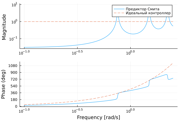
Let's construct a logarithmic amplitude-phase frequency response of the predictor and compare it with the frequency response of the negative delay. which would be an ideal controller (as a rule, such a controller cannot be implemented in practice).
C_pred = feedback(1, C0*(ss(1.0) - delay(τ))*P0)
fig_bode = bodeplot([C_pred, delay(-τ)], exp10.(-1:0.002:0.4), ls=[:solid :solid :dash :dash], title="", lab=["Smith's Predictor" "" "The perfect controller" ""])
plot!(yticks=[0.1, 1, 10], sp=1)
plot!(yticks=0:180:1080, sp=2)
Let's build a Nyquist hodograph.
fig_nyquist = nyquistplot(C * P, exp10.(-1:1e-4:2), title="τ = $τ")
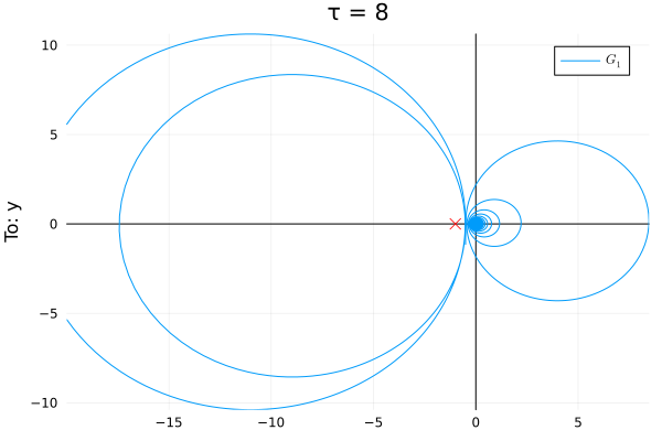
You can repeat the script by changing the delay value. τ in line 4. Note that the hodograph describes -1 at τ > 2.99.
Conclusion
In this example, we have studied methods for designing time-delayed object management systems using the Smith predictor. We also reviewed various methods of analyzing such systems and their visualization.