Modeling of control systems using the example of a PID controller
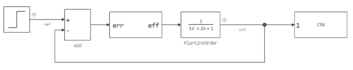
In this example, we will consider the control of a stable second-order object using a PID controller in the Engee environment. Additionally, the simulation results in the Engee environment will be compared with the simulation results in Simulink.
The control system under study is located in the pid_controls_tf_stable.engee model:
Preparation and setup
Connect the necessary libraries and run Simulink:
Pkg.add(["Statistics"])
using Plots
using MATLAB
using Statistics
gr( fmt=:png )

mat"start_simulink"
Modeling in Engee
To run the model in Engee, we need to perform the following sequence of actions:
- Upload the model using the Engee API
- Run the simulation using the same API
modelName = "pid_controls_tf_stable";
PID_model = modelName in [m.name for m in engee.get_all_models()] ? engee.open( modelName ) : engee.load( "$(@__DIR__)/$(modelName).engee");

results = engee.run( modelName )
We will extract the data for their analysis:
PID_res_e_t = results["out"].time;
PID_res_e_d = results["out"].value;
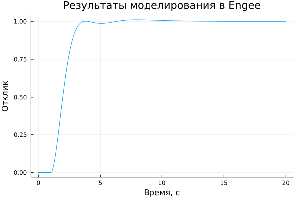
Let's build a graph for the simulation results:
plot(PID_res_e_t , PID_res_e_d, legend = false)
plot!(title = "Simulation results in Engee", ylabel = "Response", xlabel="Time, c")
Running simulations in Simulink
The library is used for communication between Engee and MATLAB MATLAB.jl. The command is responsible for calling MATLAB scripts and commands mat. To run the simulation, use the command sim:
mat"cd $(@__DIR__)"
mat"out = sim('pid_controls_tf_stable');";
In order to upload the simulation results to Engee, you first need to disassemble the object. out class Simulink.SimulationData (and don't forget to delete unnecessary data!):
mat""" res = out.yout;
       sig = res.getElement(1);
       assignin('base',sig.Name,sig.Values)
       clear res sig
   """
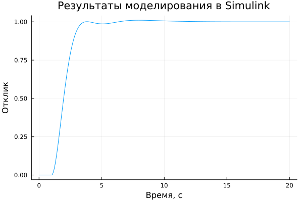
Let's look at the simulation results in Simulink:
pid_values = mat"traj.Data";
pid_times = mat"traj.Time";

plot(pid_times, pid_values, legend = false)
plot!(title = "Simulation results in Simulink", ylabel = "Response", xlabel="Time, c")
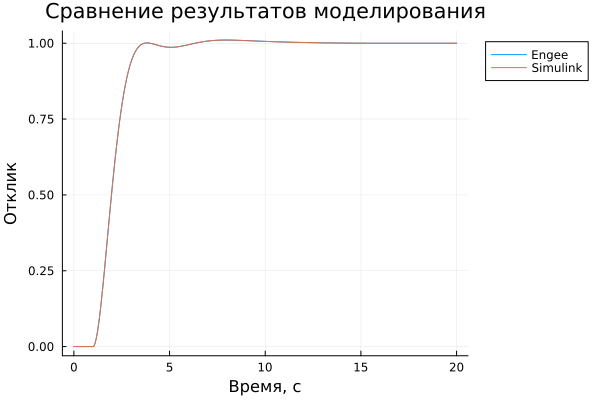
Comparison of simulation results
Let's compare the simulation results in Engee and Simulink. First, we will overlay the graphs of the results on top of each other:
plot(PID_res_e_t,PID_res_e_d, label = "Engee")
plot!(title = "Comparison of simulation results")
plot!(pid_times, pid_values, label = "Simulink")
plot!(legend = :outertopright,ylabel = "Response", xlabel="Time, c")
Then, we calculate the discrepancy between the simulation results. To do this, we will use both absolute and relative average errors of calculations, as well as correlation:
println("Correlation: ", cor(pid_values, PID_res_e_d))
The correlation is close to unity, that is, the two vectors characterizing the results in Simulink and Engee have a very strong statistical relationship, in other words, they are very close in values, now we calculate the errors.
Also, for clarity, we will plot the absolute error graph to visualize the error for the entire simulation time.
difference = pid_values - PID_res_e_d;
plot(difference)
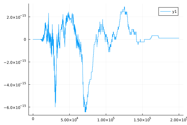
println("Average absolute error of calculations: ", abs(mean(difference)));
println("Average relative error of calculations: ", abs(mean(filter(!isnan,(difference)./pid_values)))*100, "%:");
As we can see, the calculation error is extremely small.
Conclusions
In this example, we examined the possibilities of controlling a stable second-order object using a PID controller in the Engee environment. We also made sure that Engee is comparable in accuracy to Matlab.