Simulation of an anti-lock braking system
This example will demonstrate the simulation of an anti-lock braking system (ABS). The model simulates the dynamic behavior of a vehicle under severe braking conditions and consists of a single wheel that can be reproduced several times to create a model of a multi-wheeled vehicle.
General view of the model:
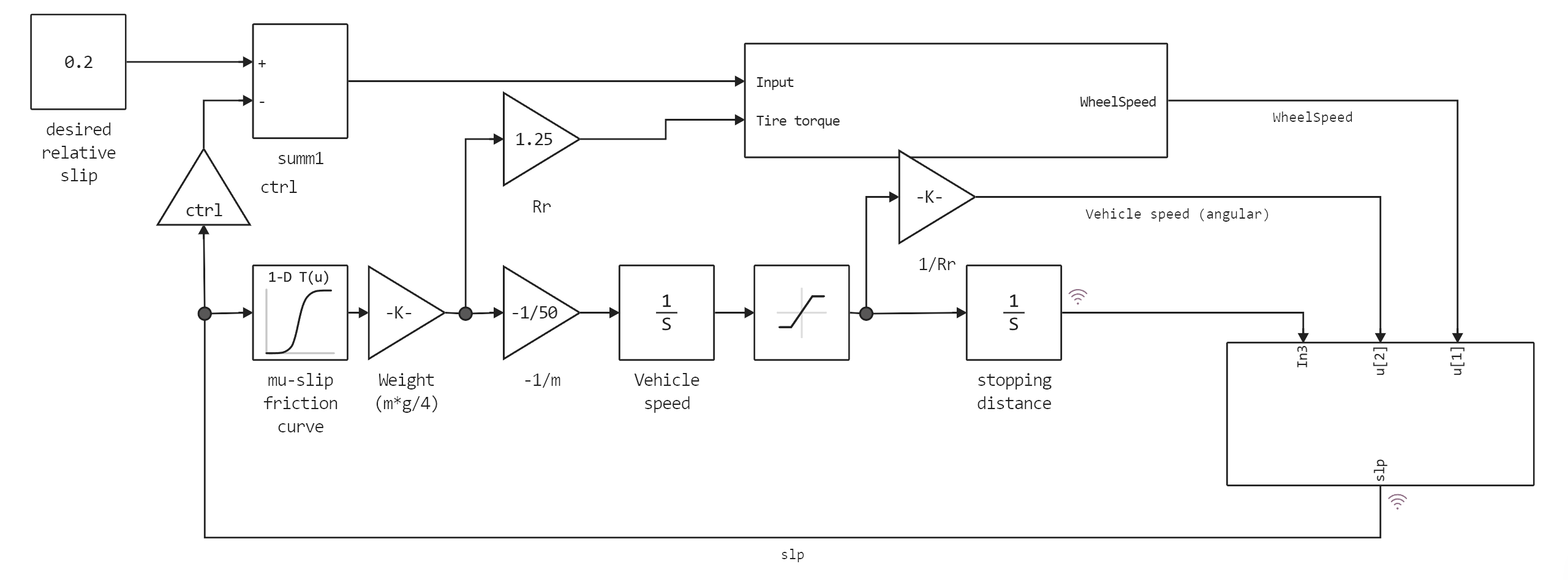
The wheel rotates at an initial angular velocity, which corresponds to the speed of the vehicle before pressing the brake pedal. To calculate the slippage, which is defined in the block of equations, we use two speeds. The speed of the vehicle is expressed as angular velocity.
(equal to the angular velocity of the wheel, if there is no slip)
Block of equations
where:
- - the speed of the vehicle divided by the radius of the wheel,
- - linear speed of the vehicle,
- - wheel radius,
- - the angular velocity of the wheel.
From these expressions, we can see that the slip is zero when the wheel speed and vehicle speed are equal, and the slip is one when the wheel is locked. The target slip value is 0.2, which means that the number of revolutions of the wheel should be 0.8 times higher than the number of revolutions in non-braking mode at the same vehicle speed. This maximizes the tire's grip on the road and minimizes braking distance when there is friction.
The coefficient of friction between the tire and the road surface, mu, is an empirical sliding function known as the mu-slip curve. We created mu-slip curves by passing MATLAB variables to a flowchart using the Simulink lookup table. The model multiplies the coefficient of friction, mu, by the weight of the wheel to obtain the friction force acting on the circumference of the tire. The friction force is divided by the mass of the vehicle to obtain deceleration, which the model integrates to obtain speed.
In this model, we used an ideal anti-lock braking controller that uses control based on the difference between actual and desired slippage. We set the desired slip to the amount of slip at which the mu-slip curve reaches its maximum value, which is the optimal value for the minimum stopping distance (see note below).
Note: In a real vehicle, the slip cannot be measured directly, so this control algorithm is impractical. In this example, it is used to illustrate the conceptual construction of such a simulation model. The real engineering value of such modeling is to show the potential of a management concept before addressing specific implementation issues.
Starting the model with the ABS enabled
Enabling the backend method for displaying graphics:
using Plots
gr()
Initial conditions that determine whether the ABS is turned on or off:
ctrl = 1.0; # ABS is enabled
Loading and launching the model:
try
    engee.close("absbrake", force=true) # closing the model
    catch err # if there is no model to close and engee.close() is not executed, it will be loaded after catch.
        m = engee.load("$(@__DIR__)/absbrake.engee") # loading the model
    end;

try
    engee.run(m, verbose=true) # launching the model
    catch err # if the model is not loaded and engee.run() is not executed, the bottom two lines after catch will be executed.
        m = engee.load("$(@__DIR__)/absbrake.engee") # loading the model
        engee.run(m, verbose=true) # launching the model
    end
Extracting data describing braking distance and sliding from the simout variable:
data1 = collect(simout)
Defining data from the model into the corresponding variables:
slp1 = collect(data1[2])
stop_distance1 = collect(data1[1])
Visualization of the time slip value:
plot(slp1[:,1],slp1[:,2])
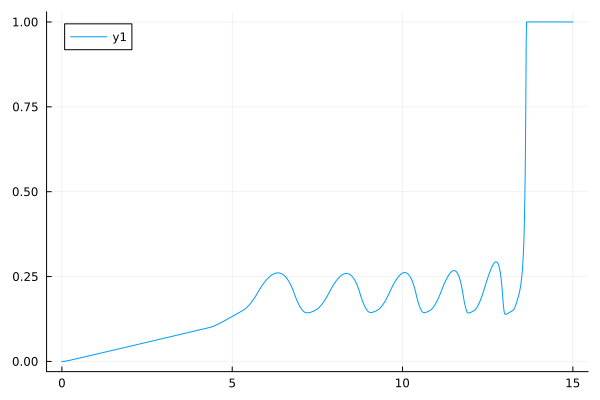
Starting the model with the ABS turned off
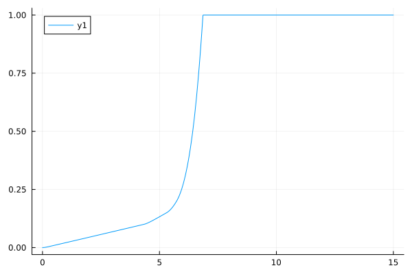
ctrl = 0.0;
Changing the model parameter:
try
    engee.close("absbrake", force=true) # closing the model
    catch err # if there is no model to close and engee.close() is not executed, it will be loaded after catch.
        m = engee.load("$(@__DIR__)/absbrake.engee") # loading the model
    end;

try
    engee.run(m, verbose=true) # launching the model
    catch err # if the model is not loaded and engee.run() is not executed, the bottom two lines after catch will be executed.
        m = engee.load("$(@__DIR__)/absbrake.engee") # loading the model
        engee.run(m, verbose=true) # launching the model
    end
Extracting data describing braking distance and sliding from the simout variable:
data2 = collect(simout)
Defining data from the model into the corresponding variables:
slp2 = collect(data2[2])
stop_distance2 = collect(data2[1])
Visualization of the time slip value:
plot(slp2[:,1],slp2[:,2])
Comparison of braking distance calculation results with and without ABS:
plotlyjs()
plot(stop_distance1[:,1], stop_distance1[:,2]./3.28084, label="Braking with ABS", xlabel="Time, from", ylabel="Stopping distance, m")
plot!(stop_distance2[:,1], stop_distance2[:,2]./3.28084, label="Braking without ABS", legend=:bottomright)
Conclusion:
In this example, the simulation of an anti-blocking system was demonstrated. A comparison of the braking distance with and without ABS has shown that braking with ABS is the most effective.