Engee documentation
Notebook

Connecting models

In this example, we will learn how to model the connection of LTI systems in Engee. From simple serial and parallel connections to complex flowcharts.

Review

Engee provides a number of functions to help you create LTI model unions. These include functions:

  • Serial and parallel connection (series, parallel)
  • Connection with feedback (feedback, feedback2dof)
  • Input and output concatenation ([ , ], [ ; ], append, array2mimo)
  • General construction of flowcharts (connect)

To illustrate the examples, we will connect the necessary libraries and create two systems with the following transfer functions:

In [ ]:
Pkg.add(["RobustAndOptimalControl", "ControlSystems"])
In [ ]:
using ControlSystems
In [ ]:
H1 = tf(2,[1, 3, 0])
Out[0]:
TransferFunction{Continuous, ControlSystemsBase.SisoRational{Int64}}
   2
--------
s^2 + 3s

Continuous-time transfer function model
In [ ]:
H2 = zpk([],[-5],5)
Out[0]:
TransferFunction{Continuous, ControlSystemsBase.SisoZpk{Int64, Int64}}
   1
5-----
 s + 5

Continuous-time transfer function model

Serial connection

Use the operator * or a function series for serial connection of LTI models, for example:
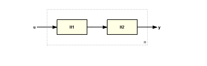
GSConnectingModels_01.png
In [ ]:
H = H2 * H1
Out[0]:
TransferFunction{Continuous, ControlSystemsBase.SisoZpk{Int64, Complex{Int64}}}
          1
10-----------------
  (s + 5)(s + 3)(s)

Continuous-time transfer function model
In [ ]:
H = series(H1,H2)
Out[0]:
TransferFunction{Continuous, ControlSystemsBase.SisoZpk{Int64, Complex{Int64}}}
          1
10-----------------
  (s + 5)(s + 3)(s)

Continuous-time transfer function model

Parallel connection

Use the operator + or a function parallel for parallel connection of LTI models, for example:
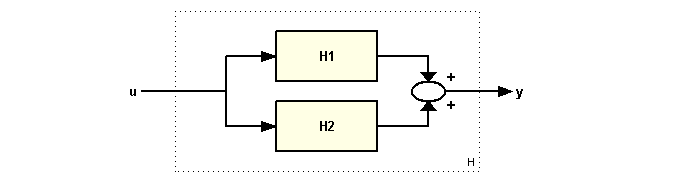
GSConnectingModels_02.png
In [ ]:
H = H1 + H2
Out[0]:
TransferFunction{Continuous, ControlSystemsBase.SisoZpk{Float64, ComplexF64}}
   (1.0s + 2.6433981132056608)(1.0s + 0.7566018867943395)
5.0------------------------------------------------------
               (1.0s + 3.0)(1.0s)(1.0s + 5.0)

Continuous-time transfer function model
In [ ]:
H = parallel(H1,H2)
Out[0]:
TransferFunction{Continuous, ControlSystemsBase.SisoZpk{Float64, ComplexF64}}
   (1.0s + 2.6433981132056608)(1.0s + 0.7566018867943395)
5.0------------------------------------------------------
               (1.0s + 3.0)(1.0s)(1.0s + 5.0)

Continuous-time transfer function model

Connection with feedback

The standard view of the structural scheme of a system with a negative feedback loop:

GSConnectingModels_03.png

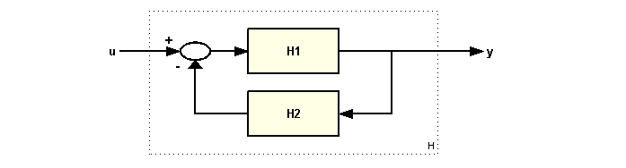
To identify a closed system, use the function feedback.

In [ ]:
H = feedback(H1,H2)
Out[0]:
TransferFunction{Continuous, ControlSystemsBase.SisoZpk{Float64, ComplexF64}}
                                    1.0s + 5.0
2.0-----------------------------------------------------------------------------
   (1.0s + 5.663076827457541)(1.0s^2 + 2.3369231725424586s + 1.7658245340262375)

Continuous-time transfer function model

Please note that feedback is negative by default. To give positive feedback, use the following syntax:

In [ ]:
H = feedback(H1, H2, pos_feedback = true)
Out[0]:
TransferFunction{Continuous, ControlSystemsBase.SisoZpk{Float64, ComplexF64}}
                                   1.0s + 5.0
2.0---------------------------------------------------------------------------
   (1.0s^2 + 8.515690830166166s + 19.3914636736468)(1.0s - 0.5156908301661673)

Continuous-time transfer function model

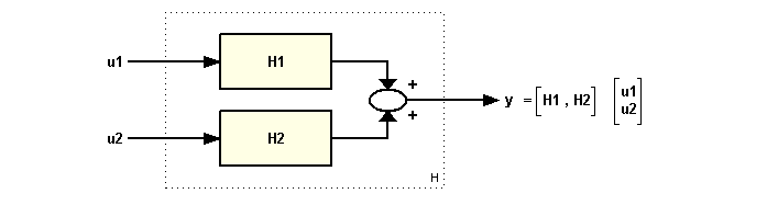
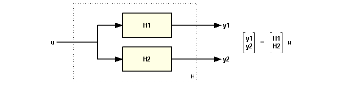
Combining inputs and outputs

You can combine the input data of the two models H1 and H2 by entering:

In [ ]:
H = [H1 H2]
Out[0]:
TransferFunction{Continuous, ControlSystemsBase.SisoZpk{Int64, Complex{Int64}}}
Input 1 to output 1
     1
2----------
 (s + 3)(s)

Input 2 to output 1
   1
5-----
 s + 5

Continuous-time transfer function model

The resulting model has two inputs and one output, which corresponds to the following scheme:

GSConnectingModels_05.png

Similarly, you can combine the output of H1 and H2 by entering:

In [ ]:
H = [ H1 ; H2 ]
Out[0]:
TransferFunction{Continuous, ControlSystemsBase.SisoZpk{Int64, Complex{Int64}}}
Input 1 to output 1
     1
2----------
 (s + 3)(s)

Input 1 to output 2
   1
5-----
 s + 5

Continuous-time transfer function model

The resulting model H has two outputs and one input and corresponds to the following flow chart:

GSConnectingModels_06.png

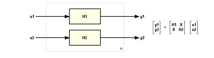
Finally, you can combine the input and output of the two models using:

In [ ]:
H = append(H1,H2)
Out[0]:
TransferFunction{Continuous, ControlSystemsBase.SisoZpk{Int64, Complex{Int64}}}
Input 1 to output 1
     1
2----------
 (s + 3)(s)

Input 1 to output 2
 1
0-
 1

Input 2 to output 1
 1
0-
 1

Input 2 to output 2
   1
5-----
 s + 5

Continuous-time transfer function model

The resulting model H has two inputs and two outputs and follows the block diagram:
GSConnectingModels_07.png

You can use concatenation to build MIMO models from elementary SISO models, for example:

In [ ]:
[H1 -tf(10,[1, 10]); 0 H2]
Out[0]:
TransferFunction{Continuous, ControlSystemsBase.SisoZpk{Int64, Complex{Int64}}}
Input 1 to output 1
     1
2----------
 (s + 3)(s)

Input 1 to output 2
 1
0-
 1

Input 2 to output 1
     1
-10------
   s + 10

Input 2 to output 2
   1
5-----
 s + 5

Continuous-time transfer function model

You can also use the function array2mimo. For example,

In [ ]:
P = ss(-1,1,1,0);
sys_array = fill(P, 2, 2) # Создает массив систем
mimo_sys = array2mimo(sys_array)
Out[0]:
StateSpace{Continuous, Int64}
A = 
 -1   0   0   0
  0  -1   0   0
  0   0  -1   0
  0   0   0  -1
B = 
 1  0
 0  1
 1  0
 0  1
C = 
 1  1  0  0
 0  0  1  1
D = 
 0  0
 0  0

Continuous-time state-space model

Building models based on flowcharts

You can use combinations of functions and operations to build models of simple flowcharts. For example, consider the following flow chart:

GSConnectingModels_09.png 
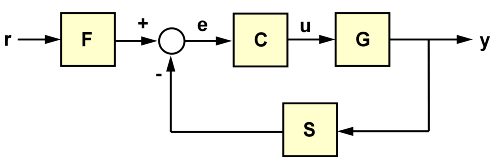
with the following data for blocks F, C, G, S:
In [ ]:
s = tf('s');
F = 1/(s + 1);
G = 100/(s^2 + 5*s + 100);
C = 20*(s^2 + s + 60)/s/(s^2 + 40*s + 400);
S = 10/(s + 10);

You can define the transfer function of a closed system from r to y as follows:

In [ ]:
T = F * feedback(G*C,S)
plot(step(T,10))
Out[0]:

But for more complex flowcharts, use the function connect libraries RobustAndOptimalControl.jl. To use connect, follow these steps:

  • Identify all the blocks in the diagram, including the summation blocks;
  • Name all the input and output channels of the blocks;
  • Match the outputs of the system blocks with the corresponding inputs of the blocks.

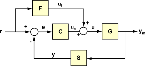
Let's look at an example of using the function using the example of the following block diagram.
GSConnectingModels_11.png

Import and connect the library RobustAndOptimalControl.jl.

In [ ]:
import Pkg
Pkg.add("RobustAndOptimalControl")
   Resolving package versions...
  No Changes to `~/.project/Project.toml`
  No Changes to `~/.project/Manifest.toml`
In [ ]:
using RobustAndOptimalControl

Use the function named_ss, in order to set the names of the input and output signals for each block.

In [ ]:
F1 = named_ss(F, x=:xF, u=:r, y=:u_f)
Out[0]:
NamedStateSpace{Continuous, Float64}
A = 
 -1.0
B = 
 1.0
C = 
 1.0
D = 
 0.0

Continuous-time state-space model
With state  names: xF
     input  names: r
     output names: u_f
In [ ]:
G1 = named_ss(G, x=:xG, u=:u, y=:y_m)
Out[0]:
NamedStateSpace{Continuous, Float64}
A = 
  0.0   16.0
 -6.25  -5.0
B = 
 0.0
 2.0
C = 
 3.125  0.0
D = 
 0.0

Continuous-time state-space model
With state  names: xG1 xG2
     input  names: u
     output names: y_m
In [ ]:
C1 = named_ss(C, x=:xC, u=:e, y=:u_c)
Out[0]:
NamedStateSpace{Continuous, Float64}
A = 
 0.0    4.0    0.0
 0.0    0.0   16.0
 0.0  -25.0  -40.0
B = 
 0.0
 0.0
 8.0
C = 
 2.34375  0.15625  2.5
D = 
 0.0

Continuous-time state-space model
With state  names: xC1 xC2 xC3
     input  names: e
     output names: u_c
In [ ]:
S1 = named_ss(S, x=:xS, u=:y_m, y=:y)
Out[0]:
NamedStateSpace{Continuous, Float64}
A = 
 -10.0
B = 
 4.0
C = 
 2.5
D = 
 0.0

Continuous-time state-space model
With state  names: xS
     input  names: y_m
     output names: y

Denote the adders using the function sumblock.

In [ ]:
Sum1 = sumblock("e = r - y")
Out[0]:
sumblock: NamedStateSpace{Continuous, Float64}
D = 
 1.0  -1.0

Continuous-time state-space model
With state  names: 
     input  names: r y
     output names: e
In [ ]:
Sum2 = sumblock("u = u_f + u_c")
Out[0]:
sumblock: NamedStateSpace{Continuous, Float64}
D = 
 1.0  1.0

Continuous-time state-space model
With state  names: 
     input  names: u_f u_c
     output names: u

It is important to mark the connections carefully. Connections are formed according to the principles that the output of one block is connected to the input of another. For example, the signal е is the output Sum1, but it is also the input for the block C.

In [ ]:
connections = [
    :e => :e # output e Sum1 to input C
    :y => :y # output y S to input Sum1
    :u => :u # output u Sum2 to input G
    :u_f => :u_f # output u_f F to input Sum2
    :u_c => :u_c # output u_c C to input Sum2
    :y_m => :y_m # output G to input S
]
Out[0]:
6-element Vector{Pair{Symbol, Symbol}}:
   :e => :e
   :y => :y
   :u => :u
 :u_f => :u_f
 :u_c => :u_c
 :y_m => :y_m

It is also important to identify the input signal w1 and a day off z1.

In [ ]:
w1 = [:r]
z1 = [:y_m]
Out[0]:
1-element Vector{Symbol}:
 :y_m

All calculated data is submitted to the input connect. You can learn more about all the function parameters in the Julia documentation Unification систем.

In [ ]:
P = connect([F1, C1, G1, S1, Sum1, Sum2], connections; w1,z1,unique = false)
Out[0]:
NamedStateSpace{Continuous, Float64}
A = 
 -1.0  0.0       0.0       0.0   0.0    0.0    0.0
  0.0  0.0       4.0       0.0   0.0    0.0    0.0
  0.0  0.0       0.0      16.0   0.0    0.0    0.0
  0.0  0.0     -25.0     -40.0   0.0    0.0  -20.0
  0.0  0.0       0.0       0.0   0.0   16.0    0.0
  2.0  4.6875    0.3125    5.0  -6.25  -5.0    0.0
  0.0  0.0       0.0       0.0  12.5    0.0  -10.0
B = 
 1.0
 0.0
 0.0
 8.0
 0.0
 0.0
 0.0
C = 
 0.0  0.0  0.0  0.0  3.125  0.0  0.0
D = 
 0.0

Continuous-time state-space model
With state  names: xF##feedback#587 xC1##feedback#587 xC2##feedback#587 xC3##feedback#587 xG1##feedback#587 xG2##feedback#587 xS##feedback#587
     input  names: r
     output names: y_m

Let us construct the transition process of the resulting closed system.

In [ ]:
plot(stepinfo(step(P,5)))
Out[0]:

Conclusion

In this article, we looked at ways to connect models. You can study the functions for converting structural diagrams in more detail in the section [Building systems] (https://engee.com/helpcenter/stable/julia/ControlSystems/lib/constructors.html ).