Conveyor management system
This example continues the development of the pipeline modeling project. Using the Engee Function and Chart blocks, we simulate the movement of loads of various weights on a belt and a conveyor control system based on a programmable logic controller (PLC). Finally, we test the physical model with the control algorithm in real time on the KPM RHYTHM.
Introduction
In the previous example of the project, we calculated and modeled the electrical and mechanical conveyor systems in conditions of varying belt loads. Now it's time to move on to automating the conveyor. At this stage of the project development, we will expand the initial model.:
-
add an engine braking system,
-
we will develop a block for calculating the position and total load of loads on the belt,
-
add subsystems:
-
determining the arrival of cargo at the edge of the belt,
-
placing new cargo on the belt,
-
-
We will develop a conveyor management system.
The example model
The model of the current example eventually looks like the one shown in the figure below.:
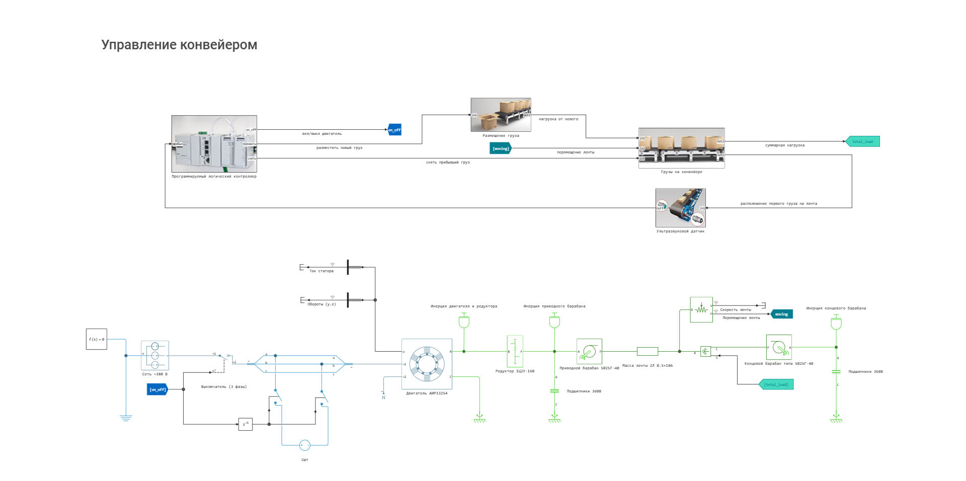
Let's consider the model elements in detail below.
Changes in the physical block chain
Dynamic braking circuits have been added to the system of physical blocks - by signal on_off The AC power supply is turned off, and in the next step of the simulation, a constant voltage is applied to the two phases of the motor from the source. Uдт.
Subsystem "Loads on the conveyor"
The main element of the subsystem "Loads on the conveyor" is the [Engee Function] block (https://engee.com/helpcenter/stable/en/base-lib-user-defined-function/engee-function.html ), in which the Julia code describes the behavior of loads on the tape during the simulation process. This unit receives signals:
-
"placement of new cargo" (variable
in1) - the duration of one simulation step, and the amount of tension of the new load being placed, -
"tape movement" (variable
in2) is the distance traveled by the conveyor belt since the start of the simulation, -
"remove incoming cargo" (variable
in3) is a logical signal that serves as a command to remove the cargo that was delivered to the edge of the tape from the description model of the goods on the tape.
At the output of the block, we receive the following signals:
-
"positions" is a static vector that contains all the values of the current location of the loads associated with the movement of the belt. At the subsystem's output, the first element corresponding to the load with the largest position value is allocated from this vector, i.e., the one standing furthest from the beginning of the belt.
-
"loads" is a vector of static size that contains all the load values from each load corresponding to the "position" vector.
-
"total load" - the total amount of load from all loads on the belt. The output of the subsystem is transmitted with a minus sign to form the correct load vector.
Below is the code from the tab Step method Code the Engee Function block with comments to explain how the subsystem works.
 if any(w -> w != 0.0, c.wght) # если на ленте есть хотя бы один груз
        idx = findfirst(w -> w == 0.0, c.wght) # находим его индекс в векторе
        c.pos[1:(idx-1)] = c.pos[1:(idx-1)] .+ (in2 - c.mov[1]) # увеличиваем перемещение каждого груза на приращение перемещения ленты
    end

    c.mov[1] = in2 # сохраняем текущее перемещение ленты

    if in3 == true # если требуется снять первый груз
        for i in 1:length(c.wght)-1 # передвигаем все грузы в векторе нагрузок на idx-1
            c.wght[i] = c.wght[i+1]
        end
        c.wght[end] = 0.0
        for i in 1:length(c.pos)-1 # передвигаем все грузы в векторе положений на idx-1
            c.pos[i] = c.pos[i+1]
        end
        c.pos[end] = 0.0
    end

    if (in1 > 0.0) && (0.0 in c.wght) # если поступает новый груз
        idx = findfirst(w -> w == 0.0, c.wght)
        c.wght[idx] = in1 # размещаем его нагрузку на вакантную позицию
        c.pos[idx] = 0.0 # задаём ему положение "0.0"
    end


    return c.pos, c.wght, sum(c.wght) # выводим: вектор положений, нагрузок, суммарную нагрузку
Variables c.pos, c.wght, sum(c.wght) they are defined in the block structure and initialized with zero values.
Subsystem "Ultrasonic sensor"
The value of the load position furthest from the beginning of the belt, calculated in the "Loads on the conveyor" block, is transmitted to the "Ultrasonic sensor" subsystem. If the load position is equal to the location of the sensor L, a high-level logical signal "load can be removed" is generated. The location of the sensor L in this example is equal to the distance between the conveyor drums.
.png)
Subsystem "Cargo placement"
Another auxiliary subsystem is "Cargo placement". In it, according to the "place a new load" signal from the programmable logic controller, a signal with a duration of one simulation step and a random load value in the range previously set in the original example is generated.
.png)
The received "load from new" signal is then sent to the "loads on the conveyor" subsystem.
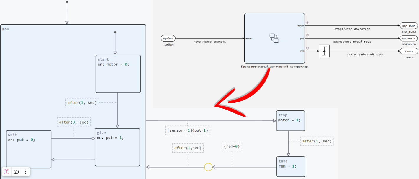
Subsystem "Programmable logic controller"
The conveyor control algorithm is defined in the Programmable Logic Controller (PLC) subsystem using the [Chart] block (https://engee.com/helpcenter/stable/en/state-machines/chart.html ).
The working principle of the algorithm is intuitive, but additionally we will fix the main points.:
-
There are 2 main processes in the state diagram:
-
Tape movement (condition
mov), -
Handling cargo removal.
-
-
Condition
movIt includes three substates:-
start- performed only at the beginning of the simulation, starts the engine (motor = 0), 1 second after it, the following state turns on: -
give- generates a load placement signal (put = 1), immediately after it, the transition to the next state is performed: -
wait- removing the load placement signal (put = 1), we form a 3-second wait for a new load to be placed.
-
-
Cargo removal is handled as follows:
-
if the load sensor is triggered (
sensor == 1), there is a transition to the statestop, -
in
stopthe engine stops (motor = 1), after 1 second, there will be a transition to the next state: -
a signal for the removal of incoming cargo is generated in take (
rem = 1), -
Immediately after that, the load removal signal is removed (
rem = 0), -
after 1 second, the chart returns to the state
mov.
-
.png)
Let's move on to modeling in Engee.
Modeling in Engee
Let's run the model using software modeling control and pre-prepared functions for ease of working with the model and simulation results:
(example_path = @__DIR__) |> cd; # We get the absolute path to the directory containing the current script and go to it.
include("useful_functions.jl"); # We connect the Julia script with auxiliary functions
simout = get_sim_results("conveyor_control.engee", example_path) # running the simulation
Simulation results - engine
We will receive and reduce the signals recorded in the model, measured on the engine:
t = thin(get_sim_data(simout, "Stator current", 1, "time"), 100);
Is = thin(get_sim_data(simout, "Stator current", 1, "value"), 100);
n = thin(get_sim_data(simout, "Revolutions (units)", 1, "value"), 100);
Let's plot these variables:
gr(fmt=:png, size = (900,400))
I_graph = plot(t, Is; label = "I(t)", title = "Stator current", ylabel = "I [A]", xlabel = "t [s]")
n_graph = plot(t, n; label = "n(t)", title = "Rotor speed", ylabel = "n [units]", xlabel = "t [s]")
plot(I_graph, n_graph)
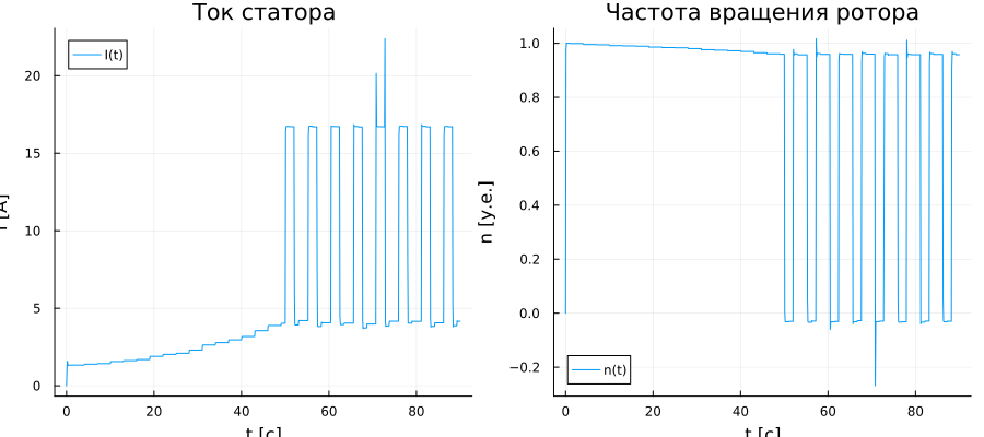
If we compare these graphs with those presented in the original example, it can be seen that when a certain load is reached on the engine, after about 50 seconds, the engine begins to stop and start periodically - it stops to remove the load. After starting the engine, the load continues to change due to the addition of new loads to the belt.
Simulation results - pipeline
We will receive and reduce the signals recorded in the model on the conveyor belt:
Vл = thin(get_sim_data(simout, "Tape speed", 1, "value"), 100);
Sл = thin(get_sim_data(simout, "Moving the tape", 1, "value"), 100);
Let's plot these variables:
V_graph = plot(t, Vл; label = "V(t)", title = "Tape speed", ylabel = "V [m/s]", xlabel = "t [s]")
S_graph = plot(t, Sл; label = "S(t)", title = "Moving the tape", ylabel = "S [m]", xlabel = "t [s]")
plot(V_graph, S_graph)
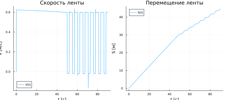
The kinematic graphs of the conveyor belt also show stops and moments where the movement does not change, which is necessary to remove the load from the belt.
Simulation results - PLC
We will receive and reduce the signals recorded in the model at the input and output of the PLC:
start_stop = thin(get_sim_data(simout, "engine start/stop", 1, "value"), 100);
rem = thin(get_sim_data(simout, "Programmable logic controller.rem", 1, "value"), 100);
pos = map(p -> p[1], thin(get_sim_data(simout, "positions", 1, "value"), 100)) .>= L;
Let's plot these variables:
plot(t, start_stop; label = "Start/Stop", width = 2, linestyle=:dot,
        title = "Controller signals", xlabel = "t [s]", legend = :outerright,
        yticks=([0, 1], ["False", "True"]), st=:steppost)
plot!(t, pos; label = "The cargo is in place", width = 1)
plot!(t, rem; label = "Remove", width = 1)
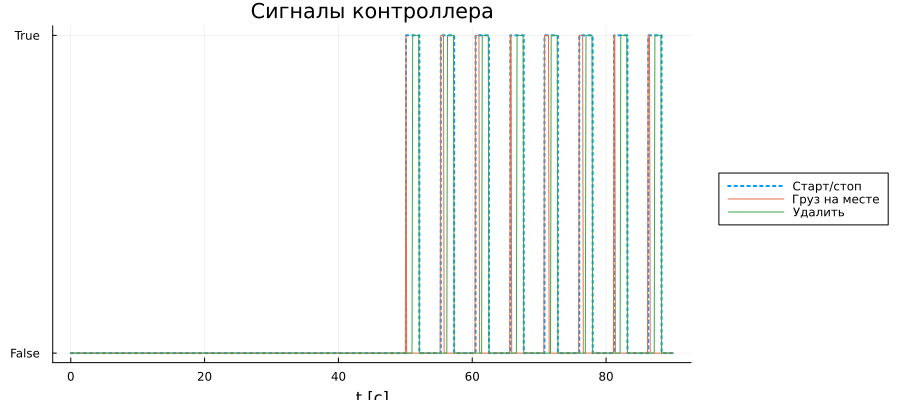
The controller receives a signal of the cargo's presence, and the controller uses this signal to generate signals of influence on the control object, according to the algorithm.
Finally, before testing the model in a system with a real PLC, we will check the operation of the model in real time.
Real-time simulation
Real-time simulation is available thanks to the integration of Engee and [real-time machine RHYTHM] (https://engee.com/community/catalogs/projects/kpm-ritm-bystryi-start ).
In [early examples](https://engee.com/community/ru/catalogs/projects/a90fd264-cf08-4c7b-93f5-350bd434fee3 It has already been shown how to simulate a control object with an assessment of its performance in hard real time. We have conducted a simulation of our facility with a control system in Engee at KPM RHYTHM, now we will evaluate TET:
Pkg.add(["StatsBase", "Printf"]) # installing the necessary packages
import StatsBase.mean, Printf.@printf # importing the required function and macro
As a result of real-time modeling, model profiling data was collected, which was subsequently recorded in a file. profile.txt . Add this data to the workspace and thin it out to save memory.
tet = TxtToVec("$(@__DIR__)/profile.txt");  # Getting a vector of values from a file
tet = filter(t -> t>0, tet);                    # Removing artifacts
thintet = thin_vector(tet, 20, 0.2);            # Thinning the vector by 95% with a deviation of up to 20%

StepTime = 1e3; # calculation step of the model, mks
Let's analyze the profiling data.
@printf "Number of profiling points: %d\n" length(tet)
@printf "Thinning: %d --> %d (%.2f %%)\n\n" l1 = length(tet) l2 = length(thintet) (l1-l2)/l1*100

@printf "Minimum TET: %.3f ms\n" tet_min = (minimum(tet)/1e6)
@printf "Average TET: %.3f ms\n" tet_mean = (mean(tet)/1e6)
@printf "Maximum TET: %.3f ms\n\n" tet_max = (maximum(tet)/1e6)

@printf "Number of TET exceedances: %d (%.2f %%)" tet_exc = count(>(StepTime*1e3), tet) tet_exc/l1*100
When evaluating TET, it was revealed that at some points the task execution time is exceeded by up to 480% relative to the calculation step. Let's build a graph of TET changes, check where such rolls appear.
gr(format = :png, legend=:bottomright, title="Model execution time\n on KPM RHYTHM",
    xlabel="Model time, ms", ylabel="Lead time, mks")


plot(thintet./1000;  label="TET", yaxis=:log, ylims=(10,1e5))
plot!([0, length(thintet)], [StepTime,  StepTime];  label="StepTime",   color=:green)
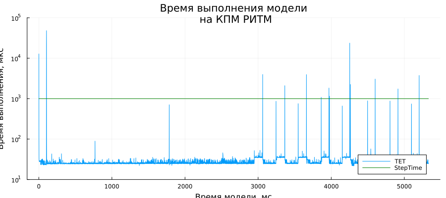
As can be seen from the TET graph, significant surges occur at certain moments of events in electrical circuits.
For the "combat" application of the model of this example, it will be necessary to refine the model to comply with real time. The following steps can be taken:
-
optimize the model,
-
Adjust the solver,
-
increase the computing power of the machine,
-
Contact the developers of the blocks that trigger events to upgrade the blocks.
Conclusion
In this example, we looked at using Engee Function and Chart to develop custom blocks and control systems. We conducted a simulation of a conveyor with cargo delivery systems and accounting for the movement of goods of various weights, as well as a prototype control system. Finally, we conducted a real-time simulation and estimated the task completion time.