Identification of a linear dynamical system
In this demo, we identify an LTI system (linear and stationary) based on the inputs and outputs of the dynamic model. This will allow us to obtain a linear model for the selected segment of data collected during the calculation of the nonlinear model, and then work with it as with a conventional linear stationary system.
Description of the model
The object of identification for us will be a model consisting of two RC filters through which rectangular pulses with a period of 0.01 s will pass.
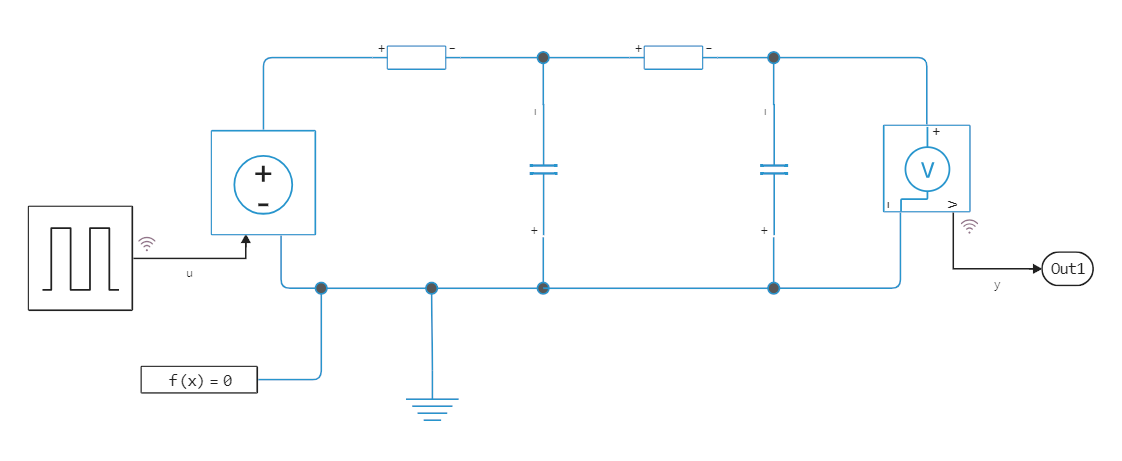
Each filter consists of a 10 ohm resistor and a 1e-04F capacitor. The input signal u it comes from the block Pulse Generator, and the output signal y is the voltage at the last capacitor of the cascade, measured by a voltmeter Voltage Sensor.
Pkg.add(["ControlSystemIdentification", "ControlSystems"])
gr()
modelName = "rc_circuit"
if !(modelName in [m.name for m in engee.get_all_models()]) engee.load( "$(@__DIR__)/$(modelName).engee"); end;
data = engee.run( modelName )
If we plot the graphs of the variables u and y then we can estimate how much the filter chain modifies the input signal. It is this behavior that we will try to describe approximately using a linear model.
t,u,y = collect(data["u"]).time, collect(data["u"]).value, collect(data["y"]).value
plot( t, [u y], label=["u" "y"] )
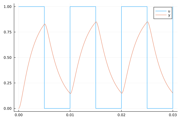
It can be expected that the aperiodic link may not be enough to accurately approximate the behavior of the system.
The identification process
We will perform the identification using the function subspaceid from the library ControlSystemIdentification:
using ControlSystems, ControlSystemIdentification
By default subspaceid returns a system in the state space of the following form:
There are more than ten other system identification functions available in the package, but it is recommended to use this one first if the system is configured in an open form. For closed-form systems, it is recommended newpem.
# We obtain the sampling frequency of the system from the time vector
Ts = t[2] - t[1]

# Let's identify the system
sys = subspaceid( iddata( y, u, Ts ));
The step response graph will allow us to evaluate the quality of the resulting model (we specifically set the pulse generator amplitude to 1, otherwise it would need to be normalized).
plot( t, y, label="The original signal" )
plot!( step( sys, 0.03 ), label="The system's reaction to the step" )
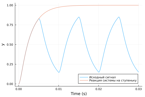
It can be seen that the reaction to a single step very accurately repeats the results of the simulation – the reaction of the initial system to rectangular pulses. If desired, we could use the second argument subspaceid limit the degree of the linear system and get a simpler, less accurate approximation.
Studying the stability of the system
Of course, the observed system is stable. But in the case of a more complex system, we could make such statements after analyzing the response, AFC, or hodographs.
A simple graph of the linear amplitude-phase-frequency response of the system can be constructed using a short function:
bodeplot( sys )
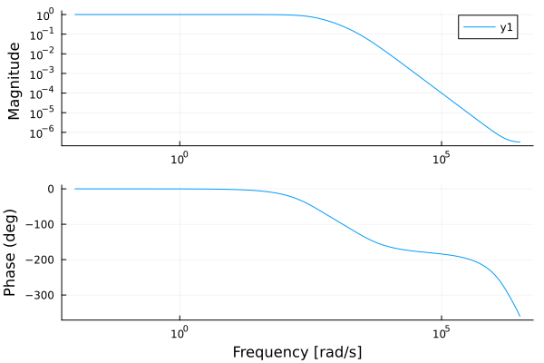
But the following code allows you to have much more control over the nature of the graph display.:
mag, phase, w = bode( sys )

plot( [w./(2pi)],
      [20*log10.( mag[:]) phase[:]], xscale=:log10, xticks=exp10.(1:8),
      linecolor=[1 2], layout=(2,1))
vline!( [1/(2Ts)  1/(2Ts)] )
plot!( title=["LFCH systems" ""], xlabel=["" "Frequency (Hz)"] )
plot!( ylabel=["Amplitude (dB)" "Phase (hail)"], leg=:false )
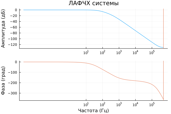
The red vertical line on them indicates a frequency equal to half the sampling frequency. The phase graph is limited to 360 degrees, but then the values of the LCF drop sharply.
Conclusion
The shown method for identifying linear models allows you to build LTI models based on a wide range of dynamic systems or simply tabular data. The resulting simplified dynamic system can be placed in a block Transfer Function and use it as a surrogate model, which is quickly calculated and, for example, allows you to study the stability of a dynamic system in the first approximation.