Car suspension simulation
This example will demonstrate the simulation of a simplified car suspension, which consists of independent front and rear vertical suspensions. The model includes the calculation of the body tilt.
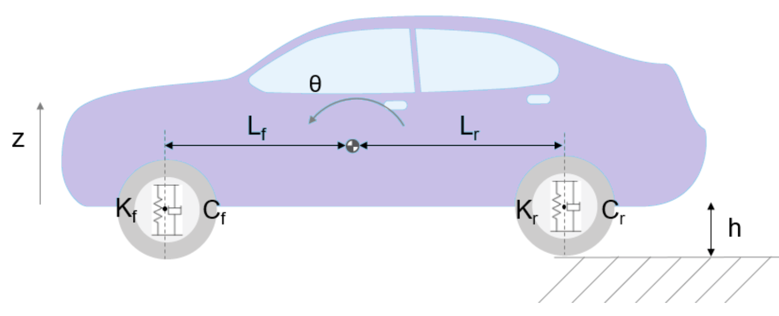
The suspension scheme of the car model:
General view of the car suspension model:
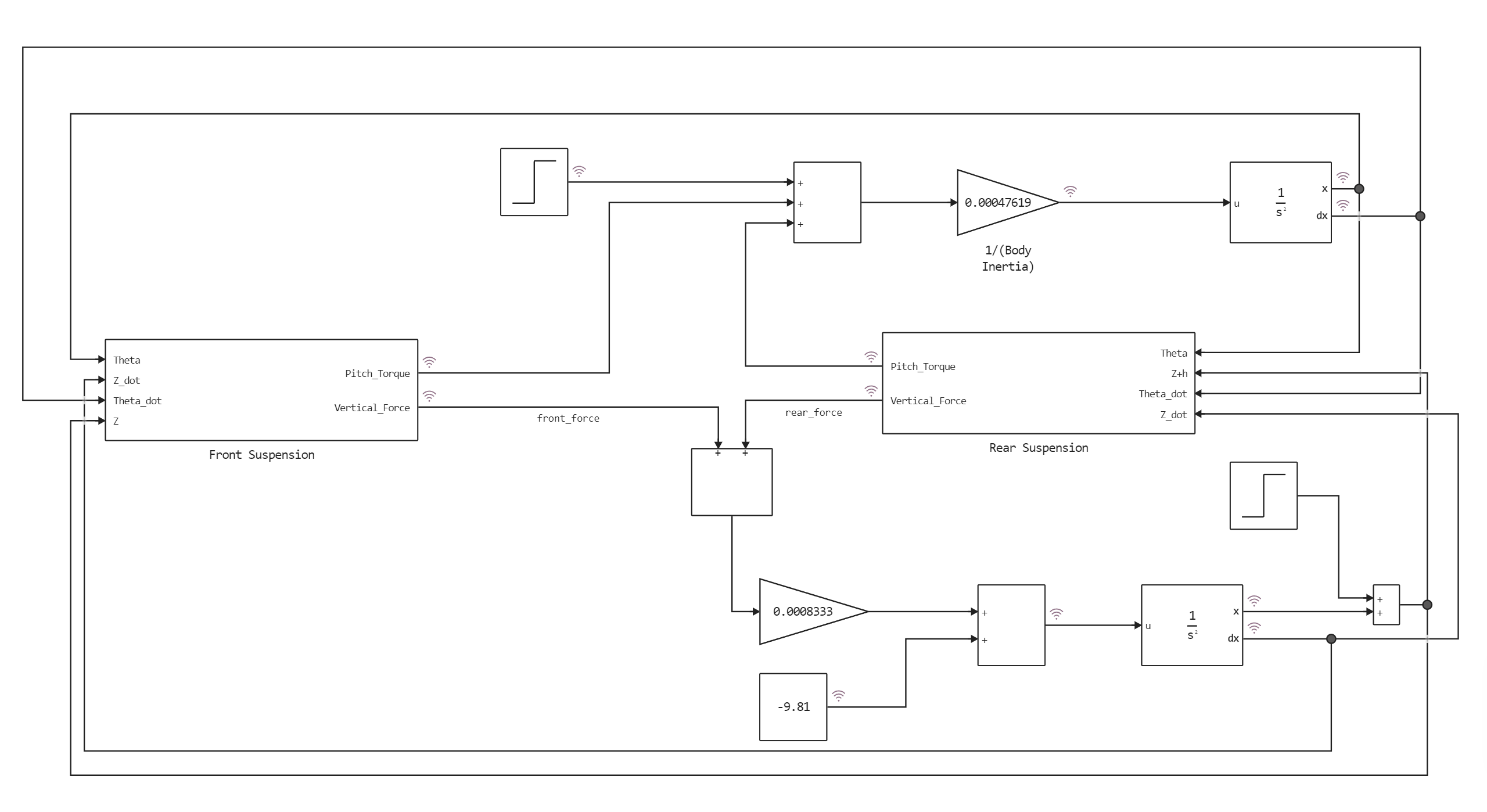
The figure shows the simulated characteristics of a half-car. The front and rear suspensions are modeled as spring-damping systems. A more detailed model would include the tire model and the non-linearities of the damper, such as velocity-dependent damping (with more rebound damping than compression). The vehicle body has degrees of freedom of tilt and bounce. They are represented in the model by four states: vertical displacement, vertical velocity, angular displacement in pitch, and angular velocity in pitch. A complete model with six degrees of freedom can be implemented using vector algebra blocks to perform axis transformations and force/displacement/velocity calculations. Equation block 1 describes the effect of the front suspension on rebound (i.e. vertical degree of freedom).:
where:
Equation block 2 describes the pitching moments caused by suspension.
where:
Equation block 3 resolves the forces and moments that arise during the movement of a body, according to Newton's Second Law.:
where:
Loading and running the simulation
Enabling the backend method for displaying graphics:
using Plots
gr();
Loading and launching the model:
try
    engee.close("suspension", force=true) # closing the model
    catch err # if there is no model to close and engee.close() is not executed, it will be loaded after catch.
        m = engee.load("/user/start/examples/controls/suspension/suspension.engee") # loading the model
    end;

try
    engee.run(m, verbose=true) # launching the model
    catch err # if the model is not loaded and engee.run() is not executed, the bottom two lines after catch will be executed.
        m = engee.load("/user/start/examples/controls/suspension/suspension.engee") # loading the model
        engee.run(m, verbose=true) # launching the model
    end
Processing of results
Extracting data describing braking distance and sliding from the simout variable:
sleep(5)
data = collect(simout)
Defining data from the model into the corresponding variables:
stop_signal = collect(data[1])
barrier_signal = collect(data[2])
front_force = collect(data[3])
angle_speed = collect(data[4])
rear_force = collect(data[5])
angle = collect(data[6]);
Visualization of simulation results:
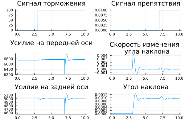
p1 = plot(stop_signal[:,1], stop_signal[:,2], title="Brake light")
p2 = plot(barrier_signal[:,1], barrier_signal[:,2], title="Obstacle signal")
p3 = plot(front_force[:,1], front_force[:,2], title="Force on the front axle")
p4 = plot(angle_speed[:,1], angle_speed[:,2], title="The rate of change of \n tilt angle")
p5 = plot(rear_force[:,1], rear_force[:,2], title="Rear axle force")
p6 = plot(angle[:,1], angle[:,2], title="Tilt angle")
plot(p1, p2, p3, p4, p5, p6, layout=(3, 2), legend=false)
Conclusion:
In this example, the simulation of a simplified car suspension was demonstrated. This model allows us to investigate the effects that occur during the operation of damping elements and suspension stiffness.