Plotting system reactions
This example shows how to plot the time and frequency characteristics of linear SISO and MIMO systems.
Building time characteristics
Let's create a third-order transfer function.
Pkg.add(["RobustAndOptimalControl", "ControlSystems"])
using ControlSystems
sys = tf([8, 18, 32],[1, 6, 14, 24])
You can plot the transient and impulse functions of the system using step() and impulse() libraries ControlSystems.jl.
plot(
    plot(step(sys,10),title="Reaction to stepwise exposure"),
    plot(impulse(sys,10),title="Reaction to an impulse"),
    layout=(2,1)
)
You can also simulate the response to an arbitrary signal, such as a sine wave, using the command lsim(). The input signal is shown in gray, and the system's response is shown in blue.lsim
t = collect(0:0.001:4);
u = sin.(10*t);

plot(lsim(sys,u',t))
plot!(t,u)
Commands for obtaining frequency and time characteristics can be used with continuous and discrete signals or models. For state space models, it is also possible to plot the reaction of a system from a given initial state.
A = [-0.8 3.6 -2.1;-3 -1.2 4.8;3 -4.3 -1.1];
B = [0; -1.1; -0.2];
C = [1.2 0 0.6];
D = -0.6;
G = ss(A,B,C,D)

t1 = collect(0:0.001:18);
u1 = fill(0,(1, 18001))
x_0 = [-1.0; 0.0; 2.0]  # initial state
plot(lsim(G, u1, t1, x0 = x_0))
Frequency characteristics
Frequency domain analysis is the key to understanding the stability and operational characteristics of control systems. The Bode, Nyquist, and Nichols graphs are three standard methods for constructing and analyzing the frequency response of a linear system. You can create these graphs using the commands ControlSystemsBase.bodeplot, ControlSystemsBase.nicholsplot and ControlSystemsBase.nyquistplot.
bodeplot(sys, label="sys",title="The Bode diagram")
nyquistplot(
    sys,
    unit_circle = true,
    Mt_circles = true,
    hz = true,
    label="sys",
    title="The Nyquist Diagram"
)
ws = exp10.(range(-2,stop=2,length=200))
nicholsplot(sys,ws)
Pole and zero maps, root hodograph
The poles and zeros of a system contain valuable information about its dynamics, stability, and performance limits. For example, consider the feedback loop in the following SISO control loop.
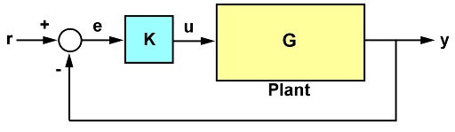
Here:
To determine the stability of a closed loop system, you can build a map of poles and zeros.
s = tf('s');
G = -(2*s+1)/(s^2+3*s+2);
k = 0.7;
T = feedback(G*k,1);

pzmap(T; hz = true)
The poles of the closed loop (marked with crosses) lie in the left half-plane, so the closed system is stable with this choice of gain.
To better understand how the reinforcement of a closed loop affects stability. You can build a graph of the location of the poles, that is, a co-root hodograph with the command rlocus().
plot(rlocus(G,3))
If we hover the cursor over the intersection of the hodograph with the Oy axis, we will see the value of the coefficient when the system becomes unstable. Thus, the gain of a closed loop must remain less than 1.5 for its stability.
Characteristics of system responses
Response graphs can display various characteristics. Let's use the example of a graph of the reaction to a stepwise effect.
result = step(T);
plot(result)
To determine the characteristics of a graph, use the function stepinfo. It returns all the characteristics of the transient process, for example, steady-state time, overshoot, and so on. This information can be written to a variable, and can also be reflected on a graph using plot.
res1 = stepinfo(result)
plot(stepinfo(result))
MIMO Systems Analysis
All the commands listed above fully support multiple input and output (MIMO) systems.
Let's create a system with two inputs and two outputs. To do this, connect the library RobustAndOptimalControl.jl.
import Pkg
Pkg.add("RobustAndOptimalControl")
using RobustAndOptimalControl
Let's define a system in the state space randomly using ssrand. Let's name the inputs, outputs, and states of the system using named_ss.
sys = named_ss(ssrand(2,2,3), x=:x, u=:u, y=:y)
sys.A .= [-0.5 -0.3 -0.2 ; 0 -1.3 -1.7; 0.4 1.7 -1.3]
sys
plot(step(sys,8))
Other useful graphs for building MIMO systems.
- The Singular Value Graph (sigma). For MIMO systems, the singular value graph shows the minimum lines on the graph corresponding to each singular value of the frequency response matrix.
- Pole/zero display for each I/O pair.
For example, plot the peak gain of sys as a function of frequency:
sigmaplot(sys)
System comparison
To compare the characteristics of different systems, you can display them on a single graph. Assign each system a specific color, marker, or line style for easy comparison. Using the feedback example above, we will construct a step-by-step closed-loop response for three values of the contour gain k in three different colors.:
k1 = 0.4;
T1 = feedback(G*k1,1);
k2 = 1;
T2 = feedback(G*k2,1);
plot(step([T T1 T2]), line=[:green :red :black])
Conclusion
In this example, we have considered the construction of various characteristics of self-propelled guns. More functions for analyzing control systems can be found in the [Analysis] section (https://engee.com/helpcenter/stable/julia/ControlSystems/lib/analysis.html ).