Investigation of the frequency characteristics of ACS
In this example, let's look at the possibilities of the Engee environment for studying the frequency characteristics of ACS.
Structural transformations
The ACS model is a structural scheme that includes blocks of typical dynamic links. The transfer function of the ACS is found using the transfer functions of these links.
When connected in series, the transfer function of the chain of links is equal to the product of their transfer functions.:
The transfer function of a group of parallel connected links is equal to the sum of their transfer functions:
If the link has a transfer function it is covered by feedback, in which there is a link , then the closed loop transfer function It is determined by the formula:
The plus or minus sign in the denominator corresponds to negative and positive feedback, respectively.
Consider the library functions ControlSystems.jl, which allow you to make structural transformations of the circuit.
Pkg.add(["ControlSystems"])
# Connect the library to work with ACS
using ControlSystems

# Setting the transfer functions
W1 = tf([1],[0.5, 1]);
W2 = tf([1],[1, 1]);
For sequential multiplication of transfer functions, there is a function ControlSystemsBase.series.
# Sequential multiplication of systems
series(W1,W2)
The transfer function of a group of parallel links can be determined using the function ControlSystemsBase.parallel.
# Parallel connection of links
parallel(W1,W2)
To determine the transfer function of a contour consisting of a link covered by feedback, there is a function ControlSystemsBase.feedback.
# If the link is covered by a single feedback, the second argument is 1
W3 = feedback(W1,1)

# If the feedback goes through the W2 link
W4 = feedback(W1,W2)

display([W3,W4])
By default, when using the function ControlSystemsBase.feedback A negative feedback connection is formed. However, you can specify that the relationship should be positive by passing -1 as the second argument.
# The link is covered by a single positive feedback
feedback(W1, -1)
Obtaining and studying the frequency characteristics of ACS
Let's set the transfer function of the ACS shown in the picture below.
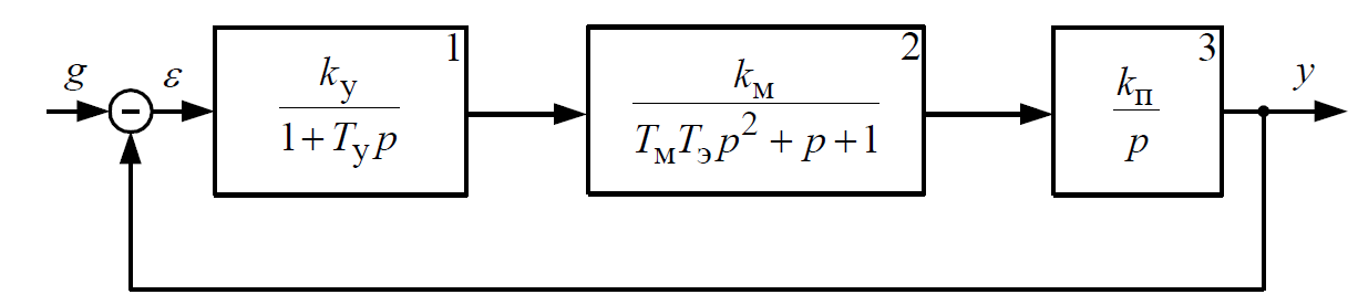
# Setting the parameters of the ACS
Ku = 10;
Tu = 0.001;
Km = 3;
Tm = 0.1;
Te = 0.02;
Kp = 0.01;
# Setting the transfer functions of the ACS links
W_1 = Ku*tf([1],[Tu, 1]);
W_2 = Km*tf([1],[Tm*Te, 1, 1]);
W_3 = Kp*tf([1],[1, 0]);

display([W_1, W_2, W_3])
The links are arranged sequentially, so we get the general transfer function of the open-loop system using the already familiar ControlSystemsBase.series.
# We obtain the transfer function of the open system
W = series(W_1, W_2)
W = series(W, W_3)
Let's plot the AFCH and LAPCH charts.
# Receiving the AFC
w = -100:0.1:100
nyquistplot(W,w,title="AFCH",label="W")
We will also construct an open-loop frequency response with a display of stability reserves in amplitude and phase. To do this, use the function ControlSystemsBase.marginplot.
# We will determine the reserves of stability by amplitude and phase
marginplot(W,label="W")
Sustainability stocks are shown in the names of the charts. The amplitude margin is 1111.76 dB, the phase margin is 73.89 degrees. The LFCH crosses 180 degrees at a frequency of 18.26 rad/s, and the cutoff frequency is 0.29 rad/s. You can also hover the cursor over the graph and view the values of amplitude, phase, and frequency at any selected point.
Conclusion
In this example, we got acquainted with the Engee functionality for studying the frequency characteristics of ACS. We also learned how to transform a block diagram using library functions. ContolSystems.jl. To learn more about plotting frequency characteristics, see Plotting functions.