RLC Circuit Response Analysis
This example shows how to analyze the time and frequency characteristics of RLC circuits depending on their physical parameters using the ControlSystems.jl functions.
Before you start, connect the package ControlSystems.jl.
import Pkg
Pkg.add("ControlSystems")
using ControlSystems
s = tf('s')
RLC Bandpass Network
The following figure shows the parallel shape of a band-pass RLC circuit.
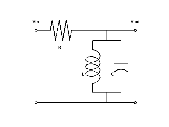
The transfer function from the input to the output voltage is:
Device controls the band frequency, and - the degree of bandwidth narrowing. To create a bandpass filter tuned to a frequency of 1 rad/s, set and use to adjust the filter band.
Analysis of the frequency response of the system
The Bode graph is a convenient tool for studying the bandwidth characteristics of an RLC network. Use tf to set the transfer function of the circuit for the values .
R = 1; L = 1; C = 1;
G = tf([1/(R*C), 0],[1, 1/(R*C), 1/(L*C)])
bodeplot(G)
As expected, the RLC filter has a maximum gain of 1 rad/s. However, the attenuation is only -10 dB, half a decade below this frequency. To get a narrower bandwidth, try increasing the value as follows.
R1 = 5;
G1 = tf([1/(R1*C), 0],[1, 1/(R1*C), 1/(L*C)]);
R2 = 20;
G2 = tf([1/(R2*C), 0],[1, 1/(R2*C), 1/(L*C)]);

bodeplot([G, G1, G2], lab = ["R = 1" "R = 5" "R = 20"])
The value of the resistor R=20 provides a narrow filter setting around the target frequency of 1 rad/s.
Analysis of the time characteristics of the circuit
We can confirm the attenuation properties of the G2 circuit (), by simulating how this filter converts sine waves with a frequency of 0.9, 1 and 1.1 rad/s.
t = 0:0.05:250;

lp1 = lsim(G2,sin.(t)',t)
lp2 = lsim(G2,sin.(0.9*t)',t)
lp3 = lsim(G2,sin.(1.1*t)',t)
plot(
    plot(lp1, title = "w = 1"),
    plot(lp2, title = "w = 0.9"),
    plot(lp3, title = "w = 1.1"),
    layout = (3,1)
)
Waves with a frequency of 0.9 and 1.1 rad/s are significantly attenuated. A wave with a frequency of 1 rad/s remains unchanged after the transient attenuation. A long transient occurs due to poorly damped filter poles, which, unfortunately, are necessary for a narrow bandwidth.
dampreport(G2)
Conclusion
Thus, we have considered which functions can be used to analyze the time and frequency characteristics of RLC circuits.