Automated control systems
This example shows how to obtain frequency response data for a SISO model of a proportional-integral controller dynamic system.
The PI controller can make the error between the desired value and the actual value become zero. This means that it can achieve precision in regulation.
Its setup is quite simple. Only two parameters need to be configured: the gain factor (Kr) and the integration time constant (Ti). With these parameters, a minimum adjustment error can be achieved.
Reference materials for some libraries:
- https://github.com/JuliaControl/ControlSystems.jl
- https://lampspuc .github.io/StateSpaceModels.jl/latest/
Pkg.add(["ControlSystems"])
# It may take about a minute to install a new library.
using ControlSystems

using Plots;
gr()
# plotlyjs() # for interactive graphs

print("Libraries are ready!")
Connect SISO systems described in the state space
P1 = ssrand(1,1,1);
P2 = ssrand(1,1,1);
append(P1, P2)
Studying the response of the transfer function
Construct the LFCS of an open and closed system $$P(s) =\frac{1}{(s+1)^4}$$ using the function gangoffourplot() to draw conclusions about the sensitivity of the system to fluctuations at different frequencies.
P = ControlSystems.tf(1,[1,1])^4
gangoffourplot( P, tf(1), titlefont = font(9), guidefont = font(8))
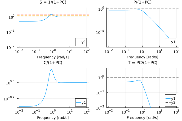
The graphs show that the system is too sensitive at frequencies around glad/s.
Setting up the PI controller
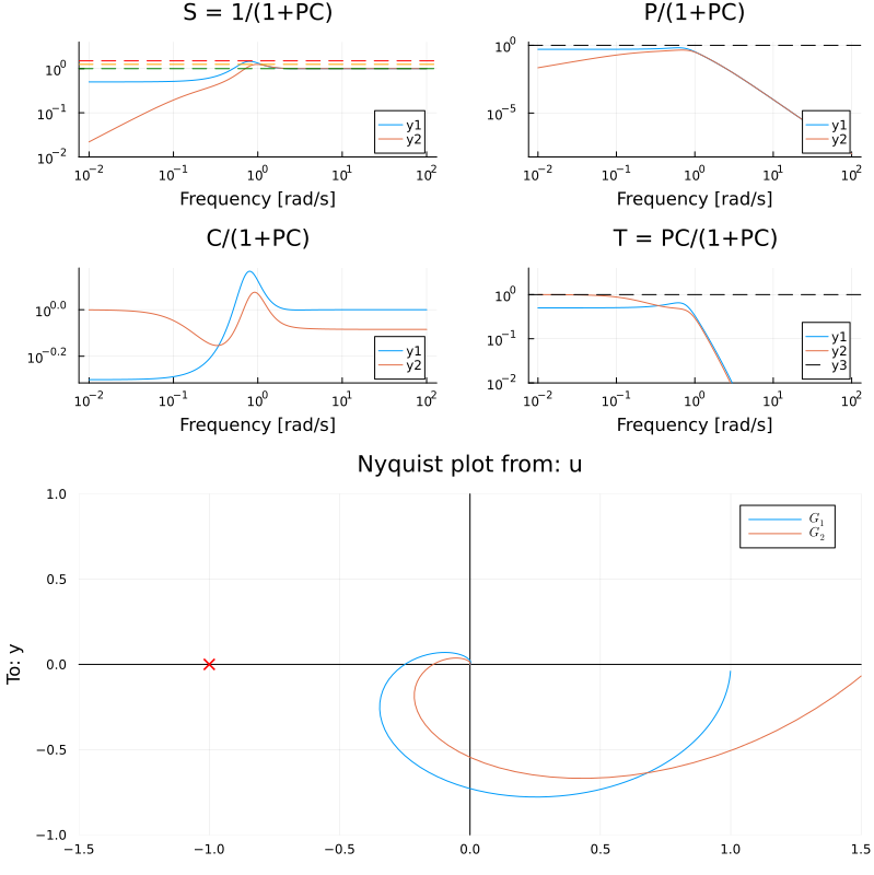
Set up the PI controller for the system $$P(s) = \frac{1}{(s+1)^4}$$
Use the function loopshapingPI, indicating that in the frequency range The rad/s system should have a 60 degree phase margin.
Output 4 graphs – LFCS for an open and for a closed system using the function gangoffourplot and the Nyquist hodograph using the function nyquistplot.
using ControlSystems, Plots

P = tf(1,[1,1])^4
ωp = 0.8
C,kp,ki = loopshapingPI(P, ωp, phasemargin=60, form=:parallel)

p1 = gangoffourplot(P, [tf(1), C]);
p2 = nyquistplot([P, P*C], ylims=(-1,1), xlims=(-1.5,1.5));

plot(p1,p2, layout=(2,1), size=(800,800))
Conclusion
In the analyzed example, an analysis of the automated control system of the PI controller was carried out.
The response of the transfer function was also studied and the PI controller was adjusted.