DC motor control
This example shows a comparison of three DC motor control methods.:
- Direct control
- Feedback management
- LQR regulation.
Let's compare these methods in terms of sensitivity to load disturbances.
Setting the task
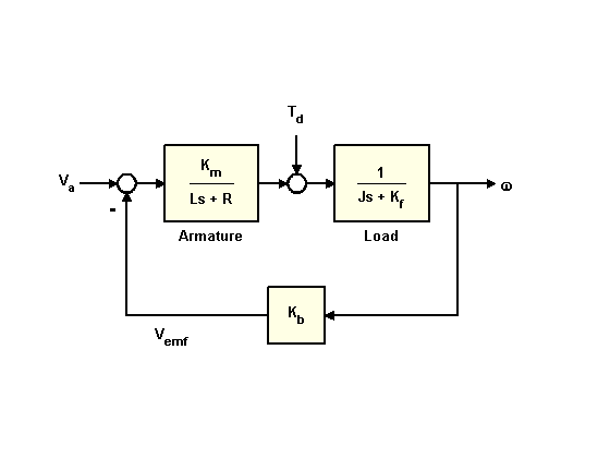
In DPT with armature control, the input voltage is controls the angular velocity of the motor shaft.
This example shows two ways to control the DPT to reduce sensitivity. load changes (changes in the torque generated by the engine load).
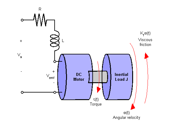
A simplified model of a DC motor is shown above. Torque parameter simulates load disturbances. It is necessary to minimize the speed fluctuations caused by such disturbances.
Let's set the engine parameters. In this example, the physical constants are:
Pkg.add(["LinearAlgebra", "RobustAndOptimalControl", "ControlSystems", "ControlSystemsBase"])
import Pkg;
Pkg.add("ControlSystemsBase")
Pkg.add("RobustAndOptimalControl")
Pkg.add("LinearAlgebra")
using ControlSystems, ControlSystemsBase, RobustAndOptimalControl, LinearAlgebra

R = 2.0 ;
L = 0.5;
Km = 0.1;
Kb = 0.1;
Kf = 0.2;
J = 0.02;
Let's build a DPT model with two inputs (,) and one exit (To begin with, we will define the description of the blocks of the block diagram presented above in the form of transfer functions.
h1 = tf([Km], [L, R])
h2 = tf([1], [J, Kf])
Let's establish a connection between the blocks. We will assign the names of the input and output signals, define the summing blocks, and establish a relationship between the blocks using the function connect().
We name the input and output signals.
H1 = named_ss(h1, x = :xH1, u = :uH1, y = :yH1)
H2 = named_ss(h2, x = :xH2, u = :uH2, y = :yH2)
Kb = named_ss(ss(Kb), x = :xKb, u = :uKb, y = :yKb)
We indicate the signals that come in and out of the summing blocks.
Sum1 = sumblock("uH1 = Va - yKb")
Sum2 = sumblock("uH2 = yH1 + Td")
We establish correspondences between the outputs and inputs of the blocks.
connections = [
    :uH1 => :uH1;
    :yH1 => :yH1;
    :uH2 => :uH2;
    :yH2 => :uKb;
    :yKb => :yKb;
]
We set the external input signals and the output signal.
w1 = [:Va, :Td]
z1 = [:yH2]
Passing the parameters to the function connect() to get a model of the systems.
dcm = connect([H2, H1, Kb, Sum1, Sum2], connections; z1, w1, verbose = true)
Now let's look at the reaction to a single step-by-step effect.
V_a = dcm[1,1];
plot(stepinfo(step(V_a,2.5)))
When applying a single step action to the input () the steady-state value of the output signal is 0.244.
Direct control of the DC motor
The first control option is direct control. We will supply the desired angular velocity value to the input system (), and also simulate the effect of an external moment () on the system.
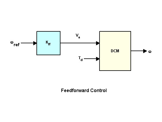
Direct communication gain factor must be set to the inverse of the DC gain from before .
Kff = 1/dcgain(V_a)[1]
To evaluate the effectiveness of a feed-forward structure in the face of load disturbances, simulate the response to a step-by-step command With indignation between seconds:
t = 0:0.01:15
Td = -0.1 * (5 .< t .< 10)
u = hcat( ones( length(t) ), Td )

cl_ff = dcm * Diagonal( [Kff, 1] )

h_1 = lsim( cl_ff, u, t )
plot( h_1, label = "Direct control, h_1(t)" )
plot!( t, Td, label = "External disturbing moment, Td" )
Feedback system
Let's consider the second control option and describe the feedback control structure.
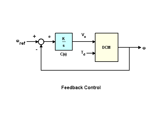
To ensure zero steady-state error, we use the controller in the form of an integrator with a gain factor.
To determine the gain K, you can use the root hodograph method applied to open-loop transmission ():
rlocusplot( ss( tf( 1, [1, 0] ) ) * V_a )
Hover over the curves to see the values of the gain and the corresponding pole. You can see that the trajectories of the two roots intersect the imaginary axis. At these points . In order for our system to remain stable, it is necessary to choose . Choose .
K = 5;
We name the input and output signals.
C = named_ss( tf( K,[1, 0] ), x=:xC, u=:e, y=:Va )
We indicate the signals that come in and out of the summing blocks.
sum = sumblock( "e = w_ref - yH2" )
We establish correspondences between the outputs and inputs of the blocks.
connections1 = [
    :e => :e;
    :Va => :Va;
    :yH2 => :yH2
]
Setting the external input signals and the output signal
w1 = [ :w_ref, :Td ]
z1 = [ :yH2 ]
Passing the parameters to the function connect() to get a model of the system.
cl_rloc = connect( [sum, C, dcm], connections1; w1, z1 )
Let's plot the output signals for direct control and feedback control.
h_2 = lsim( cl_rloc, u, t )
plot( h_1, label = "Direct control, h_1(t)" )
plot!( h_2, label = "Feedback control, h_2(t)" )
plot!( t, Td, label = "External disturbing moment, Td" )
The result of feedback control is significantly better than the direct control method. However, there are peaks at the beginning and at the end of the action .
DC motor control using a linear-quadratic regulator
To further improve performance, let's try to design a linear-quadratic regulator (LQR) for the feedback structure shown below.
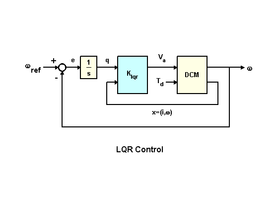
In addition to the integral, the LQR circuit also uses a state vector. for control voltage synthesis . The resulting voltage has the form
where - armature current
To better suppress disturbances, we use the cost function, which "punishes" a large integral error. For example,
where
Let's calculate the optimal LQR gain for this cost function.
Adding an exit w/s to the model dcm.
dc_aug = [ 1 ; ss( tf( 1,[1, 0] ) ) ] * V_a
We set the weight matrices Q and R, and synthesize the controller using the function lqr.
Q = [ 20 0 0; 0 1 0; 0 0 1 ]
R = 0.01
K_lqr = lqr( dc_aug, Q, R )
Then we get a closed system.
Adding an exit x using add_output(). But for this, we need the dcm variable to have the StateSpace data type, as required by the function. add_output(). Therefore, we make the conversion using ss().
dcm_new = add_output(ss(dcm), I(2))
Let's add an integrating link.
C = K_lqr * append( tf(1, [1, 0]), tf(1), tf(1) )
Description of the open-loop control system with LQR.
OL = dcm_new * append( C, ss(1) )
Description of a closed-loop control system with LQR.
CL = feedback( OL, I(3), U1=1:3, Y1=1:3 )
Transfer function (w_ref,Td)$\to$ w
cl_lqr = CL[ 1, 1:3:4 ]
Finally, let's compare the three DPT control circuits by plotting the output signals.
h_3 = lsim( cl_lqr, u, t )
plot( [h_1, h_2, h_3], label=["Direct control, h_1(t)" "Feedback control, h_2(t)" "Regulation of LQR, h_3(t)"] )
plot!( t, Td, label = "External disturbing moment, Td" )
Analyzing the graph, you can see that the peaks of the output signal have become smaller compared to the previous control method.
Conclusion
In this example, the creation of a model of a control object, a DC motor, was considered. Three methods of DPT management are compared. As a result of the analysis of the received system responses, the LQR control method proved to be the most effective and best combated the effects of an external disturbing moment.